Chapter 10 Functions
It is very important to be able to define a piece of programming logic that is repeated often. For example, I don’t want to have to always program the mathematical code for calculating the sample variance of a vector of data. Instead I just want to call a function that does everything for me and I don’t have to worry about the details.
While hiding the computational details is nice, fundamentally writing functions allows us to think about our problems at a higher layer of abstraction. For example, most scientists just want to run a t-test on their data and get the appropriate p-value out; they want to focus on their problem and not how to calculate what the appropriate degrees of freedom are. Functions let us do that.
10.1 Function Syntax
In the course of your analysis, it can be useful to define your own functions. The format for defining your own function is
where arg1, arg2, and arg3 are different arguments we will pass into the statements within the function. Arguments that are not always required (see Argument Defaults below) may be called function options. To illustrate how to define your own function, we will define a variance calculating function. Our function should take a single argument x, which should be a numerical vector. We want to perform all necessary steps of a sample variance calculation, then return the final result as a scalar.
# define my function
my.var <- function(x) {
  n <- length(x)                # calculate sample size
  xbar <- mean(x)               # calculate sample mean
  SSE <- sum( (x-xbar)^2 )      # calculate sum of squared error
  v <- SSE / ( n - 1 )          # "average" squared error
  return(v)                     # result of function is v
}
With our function composed, we can now calculate the sample variance of any numerical vector. In our abstraction, we have taken into consideration how to deal with different lengths (sample sizes) and have ensured that the function will work for any vector it is passed.
# create a vector that I wish to calculate the variance of
test.vector <- c(1,2,2,4,5)

# calculate the variance using my function
calculated.var <- my.var( test.vector )
calculated.var
## [1] 2.7Notice that even though I defined my function using the argument x and passed my function something named test.vector, R does the appropriate renaming when it performs the calculation. If my function doesn’t modify its input arguments, then R just passes a pointer to the inputs to avoid copying large amounts of data when you call a function. If your function modifies its input, then R will take the input data, copy it, and then pass that new copy to the function. This means that a function cannot modify its arguments. In Computer Science parlance, R does not allow for procedural side effects. Think of the variable x as a placeholder, with it being replaced by whatever gets passed into the function. In the example above, everywhere inside the function where an x had been written was replaced by test.vector, and the calculation proceeded properly.
Inside a function, a lot of steps might be taken and many temporary objects may be created. The goal of different functions might vary tremendously - maybe some will output a scalar like above, but other might output a matrix, data.frame, graph, even text. To ensure our function outputs the correct elements in the way we want them, it is important to properly defined a return() statement. R doesn’t completely require this and by default the a function command in R will always return the last statement. However, as code becomes more complex, it is strongly recommended (even by R’s creators) Google’s R Style Guide to always use the return() statement. Hadley Wickam’s Tidyverse Style Guide recommends not using return() except for early returns, but in the many functions I have produced for different packages over the years, nearly all of these have ended with a properly formatted data structure that is output from the function within a return() statement. Getting into this habit as you explore functions for the first time is a very good practice to get into early.
By writing a function, I can use the same chunk of code repeatedly. This means that I can do all my tedious calculations inside the function and just call the function whenever I want and happily ignore the details. Consider the function t.test() which you have likely used to do all the calculations in a t-test. We could write a similar function using the following code:
# define my function
one.sample.t.test <- function(input.data, mu0){
  n    <- length(input.data)
  xbar <- mean(input.data)
  s    <- sd(input.data)
  t    <- (xbar - mu0)/(s / sqrt(n))
  if( t < 0 ){
    p.value <- 2 * pt(t, df=n-1)
  }else{
    p.value <- 2 * (1-pt(t, df=n-1))
  }
  # lets create a string to output this
  # a string might not be a useful object to store
  # but the user might only be interested in recoring what the p-value was from the test.
  out.string <- paste('t =', round(t, digits=3), ' and p.value =', round(p.value, 3))
  return( out.string )
}
By properly formatting what I wanted output, and ensuring all details of a t-test have been thoroughly handeled, we now have our own version of a t-test function! Notice above that after I had performed all necassary calculations, I took a moment to decide how I wanted the output to be displayed. The output can be as complicated as it needs to be - my dissertation included some very LARGE list outputs from functions. Once I properly formatted what the functions output should be, the return() statement is used.
# create a vector that I wish apply a one-sample t-test on.
test.data <- c(1,2,2,4,5,4,3,2,3,2,4,5,6)
one.sample.t.test( test.data, mu0=2 )
## [1] "t = 3.157 and p.value = 0.008"Nearly every function we use to do data analysis is written in a similar fashion. Somebody decided it would be convenient to have a function that did an ANOVA analysis and they wrote something similar to the above function, but a bit grander in scope. Even if you don’t end up writing any of your own functions, knowing how to will help you understand why certain functions you use are designed the way they are. We are also only considering here the basic building blocks of a function. We haven’t done anything to ensure weird inputs are not accepted, we have not produced any unit-testing to make sure the function does not break when we make future updates, and we have not documented what the inputs and outputs of our function are. These are all very important practices to make a function robust and easy for a user to understand. We will learn more of these details in later chapters, but for now our goal is to learn how to use functions for easy and painless reproduciblity of code execution. We can worry about the more advanced details some other time!
10.2 Argument Defaults
When a function is defined it is likely it will take many arguments as inputs. It is likely that many of these arguments have common default values, so that if the user doesn’t want to worry about them, they don’t have to. To handle this, we can supply any input argument with a default. A well known statistical exmaple is the so called Standard Normal Distribution. This distribution is used in almost every introductory statistics class that is taught. For example, we might want to define a function that outputs the density of a normal curve where we can control the mean and standard deviation as input argument. But because the stanrdard normal distribution is so common, we might want to default the argument controlling the mean value to be \(0\) and the argument controlling the standard deviation to be \(1\). The user could still change these if desired, but this simplifies what is required to be supplied by a user to by only the x value of which they are interested in knowing the normal distribution density at that value.
# a function that defines the shape of a normal distribution.
# by including mu=0 and sd=1, we default he function to the standard normal
# users can always include these options with different values, and our
# function would probably incorporate those changes.
dnorm.alternate <- function(x, mu=0, sd=1){
  out <- 1 / (sd * sqrt(2*pi)) * exp( -(x-mu)^2 / (2 * sd^2) )
  return(out)
}
A user could then calculate the density of a standard normal distribution at any x value desired.
## [1] 0.2419707But maybe the normal distribution they are working with actually has mean mu = 1, so our function can handle that if they include that option within the function call.
## [1] 0.3989423Since we have a nifty function ready to go, why not use it to make a plot of the standard normal distribution. We can incorporate some of our handy dplyr functions, and quickly make a graph of the standard normal.
# Lets test the function a bit more by drawing the height
# of the normal distribution a lots of different points
# ... First the standard normal!
data.frame( x = seq(-4, 4, length=601) ) %>%
  mutate( y = dnorm.alternate(x) )       %>% # use default mu=0, sd=1
  ggplot( aes(x=x, y=y) ) + geom_line()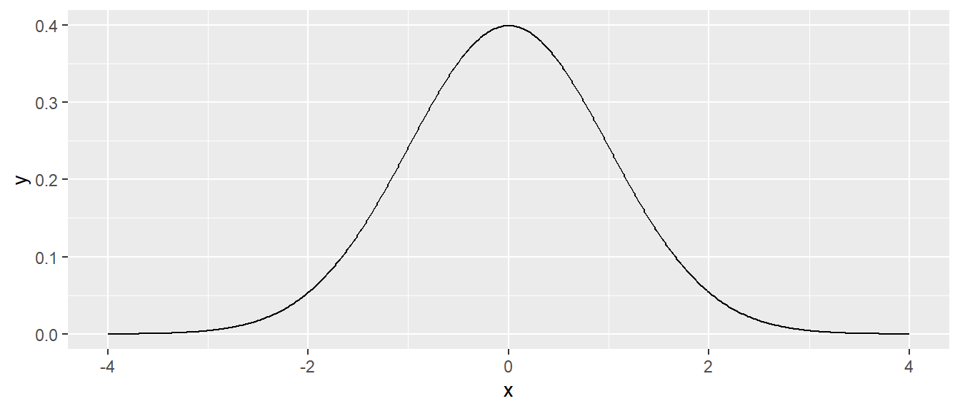
Once again though, we can change any options within our function, and the code will properly change within the function to handle this. Maybe we actually have a distribution with mean mu = 1 and sd = 0.5. Lets go ahead and include these options, and the output graph will change correspondingly.
# next a normal with mean 1, and standard deviation 1
data.frame( x = seq(-4, 4, length=601) ) %>%
  mutate( y = dnorm.alternate(x, mu=1, sd=0.5) ) %>% # use mu=1, sd=0.5
  ggplot( aes(x=x, y=y) ) + geom_line()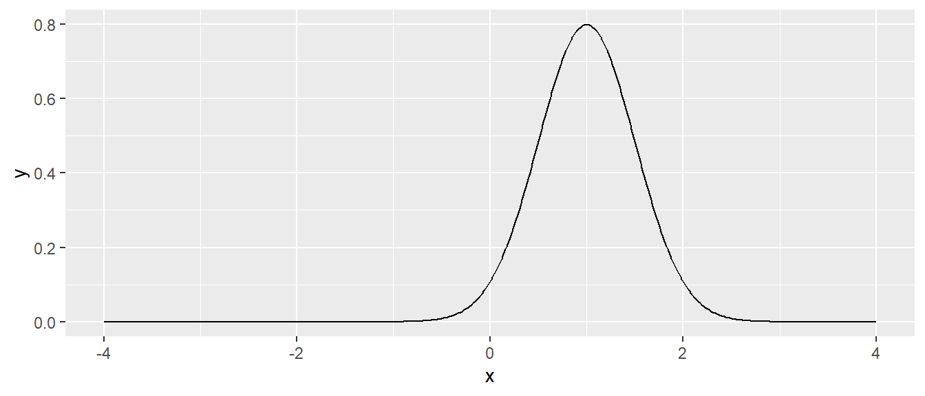
Many functions that we use have defaults that we don’t normally mess with. For example, the function mean() has an option the specifies what it should do if your vector of data has missing data. A common solution is to remove those observations and calculate the mean using only the non-NA values. However, by default, the R mean() function will indicate that the mean cannot be determine if even one NA is present in the vector. It does though have an option, na.rm, which defaults to na.rm = FALSE, but we can turn this option to TRUE by adding it to the function call.
x <- c(1,2,3,NA,5)   # fourth element is missing
mean(x)              # default is to return NA if any element is NA
## [1] NA## [1] 2.75As you look at the help pages for different functions, you’ll see in the function definitions what the default values are. For example, the function mean has another option, trim, which specifies what percent of the data to trim at the extremes. Because we would expect mean to not do any trimming by default, the authors have appropriately defined the default amount of trimming to be zero via the definition trim=0.
10.3 Ellipses
When writing functions, occasionally the situation will occur where a function a() uses within it another function, say b(), and we want to pass an unusual parameter to that function. To do this, we use a set of three periods called an ellipses. What these do is represent a set of parameter values that will be passed along to a subsequent function, but do not require explicit arguments to be added to do so. For example, the following code takes as an argument the result of a simple linear regression. The function then plots the data, the regression line, and confidence ribbon using the ggplot2 syntax previously discussed. But what if we want to change options within the ggplot environment while using this function? It is cumbersome to specify (and give good defaults) to every single graphical parameter that ggplot supports. Instead, use the ‘…’ argument and it is possible to pass any additional parameters to the ggplot functions.
This is a good moment to also introduce the require() syntax. By setting a package within the require() command, this package is used within the function, but does not have to be loaded into the local environment. Since we want this function to work, whether we have loaded the tidyverse suite or not, we can require() that tidyverse be used for this function. Now, even if you forget to load dplyr and ggplot2, this function will still operate properly.
# a function that draws the regression line and confidence interval
show.lm <- function(m, interval.type='confidence', fill.col='light grey', ...){
  require(tidyverse)   # this function can uses tidyverse without it being loaded!
  df <- data.frame(
    x = m$model[,2],   # extract the predictor variable
    y = m$model[,1]    # extract the response
  )
  df <- df %>% cbind( predict(m, interval=interval.type) )
  P <- ggplot(df, aes(x=x) ) +
    geom_ribbon( aes(ymin=lwr, ymax=upr), fill=fill.col ) +
    geom_line( aes(y=fit), ... ) + # passing down ellipses options!
    geom_point( aes(y=y), ... ) +
    labs(...)
  return(P)
}
This function looks daunting, but we experiment to see what it does. Lets fit a simple linear regression model using the trees data set, where we model the Volume as a function of Girth. Our function show.lm() can then accept the linear model as an argument, and create the ggplot graph as desired.
# first define a simple linear model from our cherry tree data
m <- lm( Volume ~ Girth, data=trees )

# call the function with no extraneous parameters
show.lm( m )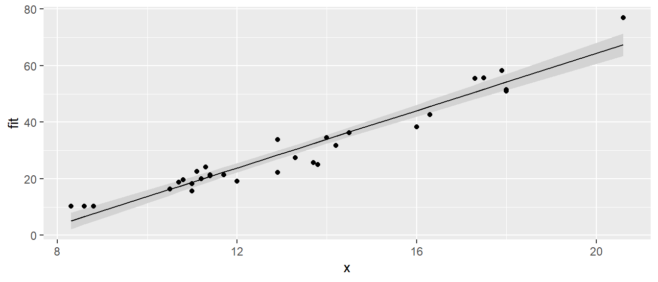
But what if we wanted to add color to the graph, maybe place a title, or do additional augmentations like those learned in previous chapters? These can be added as options to our function show.lm(), and the ellipses passes these commands onwards to the proper ggplot functions.
# Pass arguments that will just be passed along to the geom layers
show.lm( m, color='Red', title='Relationship between Girth and Volume')
## Warning in geom_line(aes(y = fit), ...): Ignoring unknown parameters: `title`## Warning in geom_point(aes(y = y), ...): Ignoring unknown parameters: `title`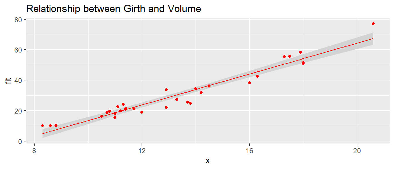
The function show.lm() has some limitations though. First, notice there were several messages printed to screen indicating that the title option is unused by certain geometries. Because we are passing the ellipses to several ggplot functions, not all of them recognize the title option, and so a message is cast to screen. Secondly, what if we wanted more than one color, for say differentiating the scatter points, best fit line, and ribbon? Ellipses, while useful, have some limitations in that they cast forward all options to each location they are placed. Thus, while very useful for not having to define many additional arguments, ellipses are limited in that we cannot specifically tell geom_line() to color the points red and lab() to add a title. All options added through the ellipses are passed to each of these functions. If we wanted a finer level of control over how to color and add text, it is a better practice to make these arguments of our function show.lm() and explicitly place them into the ggplot functions.
Do not let this deter you though, ellipses are simple and effective in the right scenarios. This type of trick is done commonly. Look at the help files for hist() and qqnorm() and you’ll see the ellipses used to pass graphical parameters along to sub-functions. Functions like lm() use the ellipses to pass arguments to the low level regression fitting functions that do the actual calculations. By only including these parameters via the ellipses, must users won’t be tempted to mess with the parameters, but experts who know the nitty-gritty details can still modify those parameters. They are worth using in many cases, but like all things, they have pros and cons.
10.4 Function Overloading
Frequently the user wants to inspect the results of some calculation and display a variable or object to the screen. The print() function does exactly that, but it acts differently for matrices than it does for vectors. It it has really unique behaviors for lists that are obtained from a call like lm() or aov(). The reason that the print function can act differently depending on the object type that it is passed is because the function print() is overloaded. What this means is that there is actually a function being used called print.lm(), and when we send an object created from lm() to the print() command, R inherently gains the properties of the object and knows to use the print.lm() function. This type of behavior is very common in R, and there are actually several hundred versions of the print() command for different types of modeling and features - a few that come to mind are print.glm() and print.gam(). Almost all well developed packages, where after a significant amount of work a user will want to view results, has its own unique overloaded print() command!
Recall that we initially introduced a few different classes of data: Numerical, Factors, and Logicals. It turns out that I can create more types of classes.
## [1] "histogram"## [1] "lm"Another commonly overloaded function is the plot() command. When you call the plot function with an lm() object, it will in turn call plot.lm() or plot.histogram() as appropriate. When building statistical models, we are often interested in different quantities and would like to get those regardless of the type of model being used. Below are a list of functions that work whether the model is fit via aov(), lm(), glm(), or gam().
| Quantity | Function Name |
|---|---|
| Residuals | resid( obj ) |
| Model Coefficients | coef( obj ) |
| Summary Table | summary( obj ) |
| ANOVA Table | anova( obj ) |
| AIC value | AIC( obj ) |
For the residual function, there exists a resid.lm() and a resid.gam(), and it is these functions that are called when we run the command resid( obj ). Although this is not the level of functions one is likely to develop frequently, it is very useful knowledge to be aware of how overloading works and that it exists. Although there is nothing that stops of us from coding in the specific resid.lm() command, it makes syntax simpler to recognize that if you want the residuals of a any type of model, we can use the resid() command, and R will inherently choose the correct overloaded version based on the properties of the object.
10.5 Debugging
When writing code, it is often necessary to figure out why the written code does not behave in the manner the writer expects. This process can be extremely challenging, and while we all hope our code is always perfect, happens on a more frequent basis than anyone wants to probably admit. Various types of tools have been developed and are incorporated in any reasonable integrated development environment (IDE) - this includes RStudio! All of the techniques we’ll discuss are intended to help the developer understand exactly what the variable environment is like during the code execution, pinpoint the syntax that is causing problems, and improve the code accordingly. These steps are often referred to as debugging.
RStudio has a support article about using the debugger mode in a variety of situations so these notes will not go into extreme detail about different scenarios. Instead we’ll focus on how one might go about debugging code.
10.5.1 Rmarkdown Recommendations
Rmarkdown documents are knitted using a completely fresh instance of R and it is highly recommend that whenever you start up RStudio, it starts with a completely fresh instance of R. This means that it should not load any history or previously created objects. To make this the default behavior, go to the RStudio -> Preferences on a Mac or Tools -> Global Options on a PC. On the R General section un-select all of the Workspace and History options. This way we can control what is loaded each time RStudio is opened. In practice, I also make a habit of never saving the .Rhistory file, which is the pop-up you see each time you try to close Rstudio.
10.5.2 Step-wise Execution
Often we can understand where an error is being introduced by simply running each step individually and inspecting the result. This is where the Evironment tab in the top right panel (unless you’ve moved it…) becomes helpful. By watching how the objects of interest change as we step through the code, we can more easily see where errors have occurred. For complicated objects such as data.frames, I find it helpful to have them opened in a View tab on a separate monitor or use the drop-down toggle to see all of the variables using the carrot toggle (a light blue arrow) next to the object name in the environment tab.
Lets consider producing a summary of the iris data set. Here is a common pipeline ending with the mean Sepal and Petal areas for each species.
iris.summary <- iris %>%
  mutate(Sepal.Area = Sepal.Width * Sepal.Length,
         Petal.Area = Petal.Width * Petal.Length) %>%
  select(Species, Sepal.Area, Petal.Area) %>%
  group_by(Speces) %>%
  summarize( Mean.Sepal.Area = mean(Sepal.Area),
             Mean.Petal.Area = mean(Petal.Area) )
In this case, the idea of step-wise execution would be to execute one section of the pipeline at a time, adding one command after another until finally the line of code that produces the error is found. I have specifically left a small - maybe difficult - error in the code above for you to try and find and fix. Once the line containing the error has been identified, one can look for misspellings, misplaced parentheses, or any other syntax problems that may be causing a disconnect between what the input structure is versus what the code expects. Can you fix the error above?
10.5.3 Print Statements
Once we start writing code with loops and functions, a simple step-by-step evaluation will no longer suffice. An easy way to quickly see what the state of a variable is at some point in the code add a print() command that outputs some useful information about the environment.
#' Compute a Factorial. e.g. 5! = 5*4*3*2*1
#' @param n A positive integer
#' @return The value of n!
factorial <- function(n){
  output <- NULL
  for( i in 1:n ){
    output <- output*i
  }
  return(output)
}

factorial(5)
## integer(0)In this case, I would add a few print statements such as the following:
#' Compute a Factorial. e.g. 5! = 5*4*3*2*1
#' @param n A positive integer
#' @return The value of n!
factorial <- function(n){
  output <- NULL
  print(paste('At Start and output = ', output))
  for( i in 1:n ){
    output <- output*i
    print(paste('In Loop and i = ', i,' and output = ', output))
  }
  return(output)
}

factorial(5)
## [1] "At Start and output = "
## [1] "In Loop and i = 1 and output = "
## [1] "In Loop and i = 2 and output = "
## [1] "In Loop and i = 3 and output = "
## [1] "In Loop and i = 4 and output = "
## [1] "In Loop and i = 5 and output = "## integer(0)Hopefully we can now see that multiplying a NULL value by anything else continues to result in NULL values. So really, output should start with the assigned value of \(0\) instead, since \(0! = 1\) would be a logical starting point for our factorial calculation, and the purpose of this function would be to calculate the factorial value of any integer \(1\) or greater.
10.5.4 browser
Debugging is best done by stepping through the code while paying attention to the current values of all the variables of interest. Modern developer environments include a debugger which allows you to step through your code, one command at a time, while simultaneously showing you the variables of interest. To get into this environment, we need to set a breakpoint. This can be done in R-scripts by clicking on the line number. In Rmarkdown files, it is done by including the command browser() into your code. The browser() function is also tremendously helpful when trying to debug a complex function, as it will allow you to step through the internal workings of the function one step at a time.
In our factorial function, we can set a break point via the following
#' Compute a Factorial. e.g. 5! = 5*4*3*2*1
#' @param n A positive integer
#' @return The value of n!
factorial <- function(n){
  browser()
  output <- NULL
  for( i in 1:n ){
    output <- output*i
  }
  return(output)
}

# Now run the function
factorial(5)
Notice that if you execute the code above, as soon as we call our function using the factorial(5) command, the browser executes in the console environment. This allows us to step through the function while simultaneously keeping track of all the variables we are interested in. You can keep click the next option, and see how the code evolves as the function is executed. As mentioned above, one might then notice that the object output never seems to update from an empty object - which might clue you into that assigning this NULL was a mistake.
10.6 Scope
Consider the case where we make a function that calculates the trimmed mean. One implementation of such a function is given here. Included is some additional syntax to help us document what the function does. We will cover such ideas in a later chapter, but it is never to early to see how a well written function should look.
#' Define a function for the trimmed mean
#' @param x A vector of values to be averaged
#' @param k The number of elements to trim on either side
#' @return A scalar
trimmed.mean <- function(x, k=0){
  x <- sort(x)      # arrange the input according magnitude
  n <- length(x)    # n = how many observations
  if( k > 0){
    x <- x[c(-1*(1:k), -1*((n-k+1):n))]  # remove first k, last k
  }
  tm <- sum(x) / length(x)  # mean of the remaining observations
  return( tm )
}
We can then create an object x, a vector of numerical values, and execute the function using this object.
## [1] 6## [1] 10 9 8 7 6 5 4 3 2 1 50Notice that even though I passed x into the function and within the function the variable x is sorted, the locally stored object x remained unsorted outside the function. When I modified x, R made a copy of x and sorted the copy that belonged to the function. It does this to purposely ensure that no modifications of a variable happens to objects that were defined outside of the scope of a function.
But what if we didn’t bother with passing x and k into the function. If we don’t pass in the values of x and k, then R will try to find them in my local environment.
# a horribly defined function that has no parameters
# but still accesses something called "x"
trimmed.mean <- function(){
  x <- sort(x)              # Access global x, sort and save in local environment
  n <- length(x)
  if( k > 0){               # Accessing the Global k
    x <- x[c(-1*(1:k), -1*((n-k+1):n))]
  }
  tm <- sum(x)/length(x)
  return( tm )
}

x <- c( 50, 10:1 )    # data to trim
k <- 2

trimmed.mean()  # amazingly this still works

# but what if k wasn't defined?
rm(k)           # remove k
trimmed.mean()  # now the function can't find anything named k and throws and error.
So if I forget to pass some variable into a function, but it happens to be defined outside the function, R will find it. It is not good practice to rely on R to do this. What if what we really wanted to do was find the trimmed mean of a vector named z? Worse yet, what if the variable x changes between runs of your function? What should be consistently giving the same result would instead keep changing! This is especially insidious when you have defined most of the arguments the function uses, but missed one. Your function happily goes to the next higher scope and sometimes finds it. I have found in my work this to be more of a curse then a blessing.
When executing a function, R will have access to all the variables defined in the function, all the variables defined in the function that called your function, and so on until the base work space. However, you should never let your function refer to something that is not either created in your function or passed in via a parameter. One good way to debug such behavior is once you believe your function is ready and all elements are properly defined, clear your local environment and pass in a new object with a ridiculous, unlikely to have been used object name like sillyvector. If the function properly executes with a cleared environment with input arguments that it should have never seen before, you have likely developed the function properly and all execution should occur within the scope of the function. We do not typically want a function to relying on any information at any other scope level outside of the function itself.
10.7 When Should I…
When a person is first learning how to program, it is a bit confusing when to write loops or functions or just divide up your code into separate blocks or scripts. The following outlines some thinking to go through when deciding whether to write code blocks, loops, or functions.
Code blocks: I separate my code using white space whenever there is a distinct change in purpose. Perhaps to mark the setup steps from the core logic of whatever I’m doing. If I’m writing a statistical analysis in an Rmarkdown document, I have program chunks for each step. In this case the code in each block is highly specialized to the task and likely won’t be re-used.
Loops: Whenever I find myself needing to repeat the same code many times, instead of copy and pasting the code, I should instead write a loop. Critically this code needs to have only slight modifications for each run and those modifications need to be controllable by just a single index variable (the iterator, like
iorj). Generally, I won’t reuse a loop in another project and the task being performed is highly specialized.Functions: There are a couple of reasons I might want to write functions.
- When I need to repeatedly run the same code, but there are aspects of how the code changes that are moderately complex. With many different function parameters, we can have the code perform in many different ways.
- I need to write code that will be used in many different locations in my project and I want to give that code a name and be able to refer to it later using that name. This allows me to also pass this code along to other functions by name (functions within functions).
- My code is so complex that I need to develop tests to verify that it works in all the situations I expect it should work. (Unit testing will be covered in the Packages chapter).
- My code is supposed to work with other chunks of code and I want to clarify exactly what information is required and exactly how the result should be structured.
10.8 Exercises
Exercise 1
Write a function that calculates the density function of a Uniform continuous variable on the interval \(\left(a,b\right)\). The uniform density function is defined as
\[ f\left(x\right)=\begin{cases} \frac{1}{b-a} & \;\;\;\textrm{if }a\le x\le b\\ 0 & \;\;\;\textrm{otherwise} \end{cases} \] which looks like this
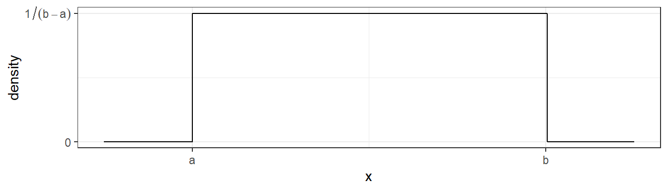
Your goal for this exercise is to write a function duniform(x, a, b) that takes an arbitrary value of x and parameters a and b and returns the appropriate height of the density function (\(1/(b-a)\)). For various values of x, a, and b, demonstrate that your function returns the correct density value.
a) Write your function without regard for it working with vectors of data. Demonstrate that it works by calling the function three times, once where \(x< a\), once where \(a < x < b\), and finally once where \(b < x\).
b) Next lets improve our function to work correctly for a vector of x values. Modify your function in part (a) so that the core logic uses a for-loop statement and the loop moves through each element of x in succession. Since this is a bit more of a complex task, your function should look something like this:
duniform <- function(x, a, b){
  output <- NULL
  for( i in ??? ){  # Set the for loop to look at each element of x
    if( x[i] ??? ){  # What should this logical expression be?
      # ???  Something ought to be saved in output[i]
    }else{
      # ???  Something else ought to be saved in output[i]
    }
  }
  return(output)
}
Verify that your function works correctly by running the following code:
data.frame( x=seq(-1, 12, by=.001) ) %>%
  mutate( y = duniform(x, 4, 8) ) %>%
  ggplot( aes(x=x, y=y) ) +
  geom_step()
c) Install the R package microbenchmark. We will use this to discover the average duration (time) your function takes to execute code. Execute the following
This will call the input R expression (your duniform function on a rather large vector of data) 100 times and report summary statistics on how long it took for the code to run. In particular, look at the median time for evaluation.
d) Instead of using a for loop, it might have been easier to use an ifelse() command, which inherently accepts vectors. Rewrite your function one last time, this time avoiding the for loop and instead introducing the vectorizable ifelse() command. Verify that your function works correctly by producing a plot of a uniform density. Finally, run the microbenchmark() code above again.
e) Comment on Which version of your function was easier to write? Which ran faster?
Exercise 2
I very often want to provide default values to a parameter that I pass to a function. For example, it is so common for me to use the pnorm() and qnorm() functions on the standard normal, that R will automatically use mean=0 and sd=1 parameters unless you tell R otherwise. This was discussed significantly in the chapter above. To get that behavior, we can set the default parameter values in the definition of a function. When the function is called, the user specified value is used, but if none is specified, the defaults are used. Look at the help page for the functions dunif(), and notice that there are a number of default parameters.
For your duniform() function provide default values of 0 and 1 for the arguments a and b. Demonstrate that your function is appropriately using the given default values by producing a graph of the density without specifying the a or b arguments.
Exercise 3
A common data processing step is to standardize numeric variables by subtracting the mean and dividing by the standard deviation. Mathematically, the standardized value is defined as
\[ z = \frac{x-\bar{x}}{s} \]
where \(\bar{x}\) is the mean and \(s\) is the standard deviation.
a) Create a function that takes an input vector of numerical values and produces an output vector of the standardized values.
b) Apply this function to each numeric column in a data frame using the dplyr::across() or the dplyr::mutate_if() commands. This is often done in model algorithms that rely on numerical optimization methods to find a solution. By keeping the scales of different predictor covariates the same, the numerical optimization routines generally work better. Below is some code that should really help once your standardize() function is working. The graphs may not look very different, but pay attention to the x- and y-axis scales!
data( 'iris' )
# Graph the pre-transformed data.
ggplot(iris, aes(x=Sepal.Length, y=Sepal.Width, color=Species)) +
  geom_point() +
  labs(title='Pre-Transformation')

# Standardize all of the numeric columns
# across() selects columns and applies a function to them
# there column select requires a dplyr column select command such
# as starts_with(), contains(), or where().  The where() command
# allows us to use some logical function on the column to decide
# if the function should be applied or not.
iris.z <- iris %>% mutate( across(where(is.numeric), standardize) )

# Graph the post-transformed data.
ggplot(iris.z, aes(x=Sepal.Length, y=Sepal.Width, color=Species)) +
  geom_point() +
  labs(title='Post-Transformation')
Exercise 4
In this exercise, you’ll write a function that will output a vector of the first \(n\) terms in the child’s game Fizz Buzz. Your function should only accept the argument \(n\), the number to which you wish to count.
Here is a description of the game. The goal is to count as high as you can but substitute in the words Fizz, Buzz or Fizz-Buzz depending on the divisors of the number. Specifically, any number evenly divisible by \(3\) should be substituted by “Fizz”, any number evenly divisible by \(5\) substituted by “Buzz”, and if the number is divisible by both \(3\) and \(5\) (i.e. by \(15\)) substitute “Fizz-Buzz”. So a sequence of integers output by your function should look like
\[
1, 2, Fizz, 4, Buzz, Fizz, 7, 8, Fizz, \dots
\]
Hint: The paste() function will squish strings together. The remainder operator is %% where it is used as 9 %% 3 = 0.
This problem was inspired by a wonderful YouTube video that describes how to write an appropriate loop to do this in JavaScript, but it should be easy enough to interpret what to do in R. I encourage you to try to write your function first before watching the video.
Exercise 5
The dplyr::fill() function takes a table column that has missing values and fills them with the most recent non-missing value. For this problem, you will create your own function to do the same.
#' Fill in missing values in a vector with the previous value.
#'
#' @parm x An input vector with missing values
#' @result The input vector with NA values filled in.
myFill <- function(x){
  # Stuff in here!
}
When you function is working properly, execute the following code that includes a call to your function.
If everything is working properly, you should obtain the output
Exercise 6
A common statistical requirement is to create bootstrap confidence intervals for a model statistic. This is done by repeatedly re-sampling with replacement from our original sample data, running the analysis for each re-sample, and then saving the statistic of interest. Below is a function boot.lm that bootstraps the linear model using case re-sampling.
#' Calculate bootstrap CI for an lm object
#'
#' @param model
#' @param N
boot.lm <- function(model, N=1000){
  data    <- model$model  # Extract the original data
  formula <- model$terms  # and model formula used

  # Start the output data frame with the full sample statistic
  output <- broom::tidy(model) %>%
    select(term, estimate) %>%
    pivot_wider(names_from=term, values_from=estimate)

  for( i in 1:N ){
    data <- data %>% sample_frac( replace=TRUE )
    model.boot <- lm( formula, data=data)
    coefs <- broom::tidy(model.boot) %>%
      select(term, estimate) %>%
      pivot_wider(names_from=term, values_from=estimate)
    output <- output %>% rbind( coefs )
  }

  return(output)
}

# Run the function on a model
m <- lm( Volume ~ Girth, data=trees )
boot.dist <- boot.lm(m)

# If boot.lm() works, then the following produces a nice graph
boot.dist %>% gather('term','estimate') %>%
  ggplot( aes(x=estimate) ) +
  geom_histogram() +
  facet_grid(.~term, scales='free')
Unfortunately, the code above does not correctly calculate a bootstrap sample for the model coefficients. It has a bug… Figure out where the mistake is and fix it! Hint: Even if you haven’t studied the bootstrap, my description above gives enough information about the bootstrap algorithm to figure this out.