Chapter 14 Transformations of random variables

14.1 Introduction

In this section we will consider transformations of random variables. Transformations are useful for:

• Simulating random variables.
  For example, computers can generate pseudo random numbers which represent draws from $U(0,1)$ distribution and transformations enable us to generate random samples from a wide range of more general (and exciting) probability distributions.
  
• Understanding functions of random variables.
  Suppose that £$P$ is invested in an account with continuously compounding interest rate $r$. Then the amount £$A$ in the account after $t$ years is
  $$A=P \text{e}^{r t}.$$ Suppose that $P=1,000$ and $r$ is a realisation of a continuous random variable $R$ with pdf $f(r)$. What is the p.d.f. of the amount $A$ after one year? i.e. What is the p.d.f. of
  $$A=1000 \text{e}^{R}?$$

We will consider both univariate and bivariate transformations with the methodology for bivariate transformations extending to more general multivariate transformations.

14.2 Univariate case

Suppose that $X$ is a continuous random variable with p.d.f. $f(x)$. Let $g$ be a continuous function, then $Y=g(X)$ is a continuous random variable. Our aim is to find the p.d.f. of $Y$.

We present the distribution function method which has two steps:

1. Compute the c.d.f. of $Y$, that is
   $$F_Y(y)=P(Y \leq y).$$
2. Derive the p.d.f. of $Y$, $f_Y(y)$, using the fact that
   $$f_Y(y)=\dfrac{dF_Y(y)}{dy}.$$

Square of a Standard Normal

Let $Z\sim N(0,1)$. Find the p.d.f. of $Y=Z^2$.

For $y>0$, the c.d.f. of $Y=Z^2$ can be expressed in terms of the c.d.f. of $Z$, $$\begin{align*} F_Y(y) &= P(Y \leq y) \\ &= P(Z^2 \leq y) \\ &= P(-\sqrt{y} \leq Z \leq \sqrt{y}) \\ &= P(Z \leq \sqrt{y}) - P(Z \leq -\sqrt{y}) \\ &= F_Z(\sqrt{y}) - F_Z(-\sqrt{y}). \end{align*}$$ Note that if we want a specific formula for $F_Y$, then we can evaluate the resulting c.d.f.’s. In this case:
$$F_Z(\sqrt{y}) = \int_{-\infty}^{\sqrt{y}} \frac{1}{\sqrt{2\pi}} e^{-\frac{z^2}{2}}dz.$$ Therefore, using the chain rule for differentiation,
$$\begin{align*} f_Y(y) &= \frac{dF_Y(y)}{dy} \\ &= \frac{d}{dy}F_Z(\sqrt{y}) - \frac{d}{dy} F_Z(-\sqrt{y}) \\ &= \frac{d}{dz} F_Z(z) \frac{d}{dy}(z) - \frac{d}{dz} F_Z(-z) \frac{d}{dy}(-z) \end{align*}$$ where $z=y^{1/2}$.
Now $\frac{d}{dz} F_Z(z) = \frac{1}{\sqrt{2\pi}} e^{-\frac{z^2}{2}}$, so $$\begin{align*} f_Y(y) &= \frac{1}{\sqrt{2\pi}} e^{-\frac{(\sqrt{y})^2}{2}} \frac{1}{2\sqrt{y}} - \frac{1}{\sqrt{2\pi}} e^{-\frac{(-\sqrt{y})^2}{2}} \frac{-1}{2\sqrt{y}} \\ &= \frac{1}{2\sqrt{2 \pi y}} e^{-\frac{y}{2}} + \frac{1}{2\sqrt{2 \pi y}} e^{-\frac{y}{2}} \\ &= \frac{1}{\sqrt{2 \pi y}} e^{-\frac{y}{2}}. \end{align*}$$ Therefore $Y$ has probability density function:
$$f_Y (y) = \left\{ \begin{array}{ll} \frac{y^{-1/2}}{\sqrt{2 \pi}} \exp \left( - \frac{y}{2} \right) \qquad & y>0, \\ 0 & \mbox{otherwise.} \end{array} \right.$$

Thus $Y \sim {\rm Gamma} \left( \frac{1}{2},\frac{1}{2} \right)$, otherwise known as a Chi-squared distribution with $1$ degree of freedom. :::

14.3 Bivariate case

Suppose that $X_1$ and $X_2$ are continuous random variables with joint p.d.f. given by $f_{X_1,X_2}(x_1,x_2)$. Let $(Y_1,Y_2)=T(X_1,X_2)$. We want to find the joint p.d.f. of $Y_1$ and $Y_2$.

Jacobian

Suppose $T:(x_1,x_2) \rightarrow (y_1,y_2)$ is a one-to-one transformation in some region of $\mathbb{R}^2$, such that $x_1 = H_1(y_1,y_2)$ and $x_2 = H_2(y_1,y_2)$. The Jacobian of $T^{-1}=(H_1,H_2)$ is defined by
$$J(y_1,y_2) = \begin{vmatrix} \frac{\partial H_1}{\partial y_1} & \frac{\partial H_1}{\partial y_2} \\[4pt] \frac{\partial H_2}{\partial y_1} & \frac{\partial H_2}{\partial y_2} \end{vmatrix} .$$

Transformation of random variables.

Let $(Y_1,Y_2)=T(X_1,X_2)$ be some transformation of random variables. If $T$ is a one-to-one function and the Jacobian of $T^{-1}$ is non-zero in $T(A)$ where
$$A=\{(x_1,x_2): f_{X_1,X_2}(X_1, X_2)>0\},$$ then the joint p.d.f. of $Y_1$ and $Y_2$, $f_{Y_1,Y_2}(y_1,y_2)$, is given by
$$f_{X_1,X_2}(H_1(y_1,y_2),H_2(y_1,y_2)) |J(y_1,y_2)|$$

if $(y_1, y_2) \in T(A)$, and $0$ otherwise.

Transformation of uniforms.

Let $X_1 \sim U(0,1)$, $X_2 \sim U(0,1)$ and suppose that $X_1$ and $X_2$ are independent. Let $$Y_1=X_1+X_2, \quad Y_2=X_1-X_2.$$

Find the joint p.d.f. of $Y_1$ and $Y_2$.

The joint p.d.f. of $X_1$ and $X_2$ is
$$\begin{align*} f_{X_1,X_2}(x_1,x_2) &= f_{X_1}(x_1)f_{X_2}(x_2) \\ &= \begin{cases} 1, \quad & \text{if } 0 \leq x_1 \leq 1 \text{ and } 0 \leq x_2 \leq 1,\\[3pt] 0, \quad & \text{otherwise.}\end{cases} \end{align*}$$ Now $T:(x_1,x_2) \mapsto (y_1,y_2)$ is defined by
$$y_1=x_1+x_2,\quad y_2=x_1-x_2.$$ Hence,
$$\begin{align*} x_1 &= H_1(y_1,y_2) = \frac{y_1+y_2}{2}, \\ x_2 &= H_2(y_1,y_2) = \frac{y_1-y_2}{2}. \end{align*}$$ The Jacobian of $T^{-1}$ is $$J(y_1,y_2) = \begin{vmatrix} \frac{\partial H_1}{\partial y_1} & \frac{\partial H_1}{\partial y_2} \\ \frac{\partial H_2}{\partial y_1} & \frac{\partial H_2}{\partial y_2} \end{vmatrix} =\begin{vmatrix} \frac{1}{2} & \frac{1}{2} \\ \frac{1}{2} & -\frac{1}{2} \end{vmatrix} = -\frac{1}{2}.$$ Since $A=\{(x_1,x_2): 0 \leq x_1 \leq 1, 0 \leq x_2 \leq 1\}$ and since the lines $x_1=0$, $x_1=1$, $x_2=0$ and $x_2=1$ map to the lines $y_1+y_2=0$, $y_1+y_2=2$, $y_1-y_2=0$ and $y_1-y_2=2$ respectively, it can be checked that
$$T(A)= \left\{ (y_1,y_2): 0\leq y_1+y_2 \leq 2, 0 \leq y_1-y_2 \leq 2 \right\}.$$

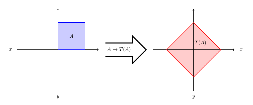
Figure 14.1: Transformation

Thus, $$\begin{align*} f_{Y_1,Y_2}(y_1,y_2) &= \begin{cases} \frac{1}{2} f_{X_1,X_2}(H_1(y_1,y_2),H_2(y_1,y_2)), & \text{if } (y_1,y_2) \in T(A),\\ 0, & \text{otherwise.}\end{cases} \\[3pt] &= \begin{cases} \frac{1}{2}, & \text{if } 0 \leq y_1+y_2 \leq 2 \text{ and } 0 \leq y_1-y_2 \leq 2,\\ 0, & \text{otherwise.}\end{cases} \end{align*}$$

Transformation of Exponentials.

Suppose that $X_1$ and $X_2$ are i.i.d. exponential random variables with parameter $\lambda$. Let $Y_1 = \frac{X_1}{X_2}$ and $Y_2=X_1+X_2$.

1. Find the joint p.d.f. of $Y_1$ and $Y_2$.
   
2. Find the p.d.f. of $Y_1$.
   

Attempt Example 14.3.4: Transformation of Exponentials and then watch Video 22 for the solutions.

Video 22: Transformation of Exponentials

Solution to Example 14.3.4

Remember from previous results that $Y_2 = X_1 + X_2 \sim {\rm Gamma} (2,\lambda)$.

1. Since $X_1$ and $X_2$ are i.i.d. exponential random variables with parameter $\lambda$, the joint p.d.f. of $X_1$ and $X_2$ is given by
   $$\begin{align*} f_{X_1,X_2}(x_1,x_2) &= f_{X_1}(x_1)f_{X_2}(x_2) \\[3pt] &= \begin{cases} \lambda e^{-\lambda x_1} \lambda e^{-\lambda x_2}, & \text{if } x_1,x_2 > 0, \\ 0, & \text{otherwise.} \end{cases} \\[3pt] &= \begin{cases} \lambda^2 e^{-\lambda(x_1+x_2)}, & \text{if } x_1,x_2 > 0, \\ 0, & \text{otherwise.} \end{cases} \end{align*}$$ Solving simultaneously for $X_1$ and $X_2$ in terms of $Y_1$ and $Y_2$, gives $X_1=Y_1X_2$ and
   $$Y_2 = X_1+X_2 = Y_1X_2 + X_2 = X_2(Y_1+1).$$ Rearranging gives $X_2 = \frac{Y_2}{Y_1+1} (=H_2 (Y_1,Y_2))$, and then $X_1 = Y_1X_2 = \frac{Y_1Y_2}{Y_1+1} (=H_1 (Y_1,Y_2))$.
   Computing the Jacobian of $T^{-1}$, we get
   $$\begin{align*} J(y_1,y_2) &= \begin{vmatrix} \frac{\partial H_1}{\partial y_1} & \frac{\partial H_1}{\partial y_2} \\ \frac{\partial H_2}{\partial y_1} & \frac{\partial H_2}{\partial y_2} \end{vmatrix} \\[3pt] &= \begin{vmatrix} \frac{y_2}{(y_1+1)^2} & \frac{y_1}{y_1+1} \\ -\frac{y_2}{(y_1+1)^2} & \frac{1}{y_1+1} \end{vmatrix} \\[3pt] &= \frac{y_2}{(y_1+1)^3} + \frac{y_1y_2}{(y_1+1)^3} \\[3pt] &= \frac{y_2}{(y_1+1)^2}. \end{align*}$$

Now,

$$\begin{align*} A &= \left\{ (x_1,x_2):f_{X_1,X_2}(x_1,x_2)>0 \right\} \\ &= \left\{ (x_1,x_2):x_1>0,x_2>0 \right\}. \end{align*}$$

Therefore, $T(A) \subseteq \left\{(y_1, y_2):y_1>0, y_2>0\right\}$. Since $x_1>0$ and $x_2>0$, $y_1=\frac{x_1}{x_2}>0.$ Furthermore, since $x_1=\frac{y_1y_2}{y_1+1}>0$, then $y_1y_2>0$ implies $y_2>0$. Therefore,

$$T(A)=\left\{ (y_1,y_2):y_1>0,y_2>0 \right\}.$$

Consequently, the joint p.d.f. of $Y_1$ and $Y_2$, $f=f_{Y_1,Y_2}(y_1,y_2)$ is given by

$$\begin{align*} f &= f_{X_1,X_2} \left( H_1(y_1,y_2),H_2(y_1,y_2) \right) \left| J(y_1,y_2) \right| \\[3pt] &= f_{X_1,X_2} \left( \frac{y_1y_2}{1+y_1},\frac{y_2}{1+y_1} \right) \left|\frac{y_2}{(1+y_1)^2} \right| \\[3pt] &= \lambda^2 e^{-\lambda \left( \frac{y_1y_2}{(1+y_1)} + \frac{y_2}{(1+y_1)} \right)} \frac{y_2}{(1+y_1)^2} \\[3pt] &= \lambda^2 e^{-\lambda y_2} \frac{y_2}{(1+y_1)^2}, \quad \text{if } y_1,y_2>0. \end{align*}$$

If either $y_1<0$ or $y_2<0$, then $f_{Y_1,Y_2}(y_1,y_2)=0$.

2. The p.d.f. of $Y_1$ is the marginal p.d.f. of $Y_1$ coming from the joint p.d.f $f_{Y_1,Y_2}(y_1,y_2)$. Therefore, for $y_1 >0$,
   $$\begin{align*} f_{Y_1}(y_1) &= \int_0^{\infty} \lambda^2 e^{-\lambda y_2} \frac{y_2}{(1+y_1)^2} dy_2 \\ &= \frac{1}{(1+y_1)^2} \int_0^{\infty} \lambda^2 y_2 e^{-\lambda y_2} dy_2 \\ &= \frac{1}{(1+y_1)^2}. \end{align*}$$ (In the above integration remember that $\lambda^2 y_2 e^{-\lambda y_2}$ is the p.d.f. of ${\rm Gamma} (2,\lambda)$.)
   So,
   $$f_{Y_1}(y_1) = \begin{cases} \frac{1}{(1+y_1)^2} & \text{if } y_1>0, \\[3pt] 0 & \text{otherwise.} \end{cases}$$ The distribution $Y_1$ is an example of a probability distribution for which the expectation is not defined.
   
   

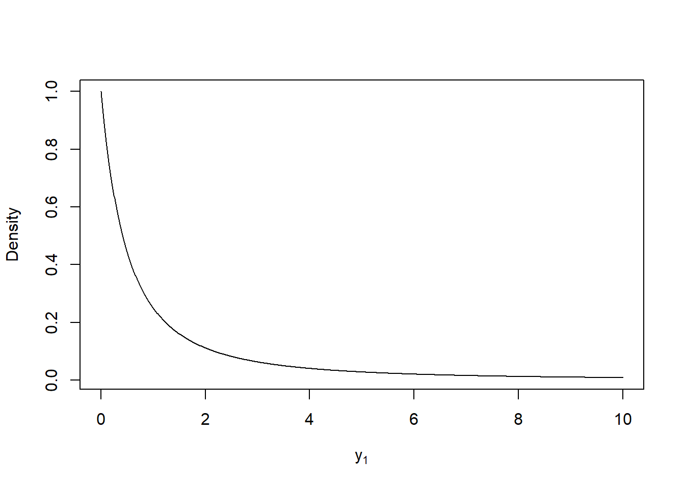
   Figure 14.2: Plot of the p.d.f. of $Y_1$.

Note that one can extend the method of transformations to the case of $n$ random variables.

Student Exercise

Attempt the exercise below.

Let $X$ and $Y$ be independent random variables, each having probability density function $$f(x) = \begin{cases} \lambda e^{-\lambda x} & \text{if } x>0, \\ 0 & \text{otherwise} \end{cases}$$ and let $U=X+Y$ and $V=X-Y$.

1. Find the joint probability density function of $U$ and $V$.
   
2. Hence derive the marginal probability density functions of $U$ and $V$.
   
3. Are $U$ and $V$ independent? Justify your answer.
   

Solution to Exercise 14.1.

1. Let the transformation $T$ be defined by $T(x,y)=(u,v)$, where $u=x+y$ and $v=x-y$. Then, $x=\frac{1}{2} (u+v)$ and $y={1\over2}(u-v)$, so that
   $$J(u,v)=\left| \begin{matrix} \frac{1}{2} & \frac{1}{2} \\ \frac{1}{2} & -\frac{1}{2} \end{matrix} \right| = -\frac{1}{2}.$$ Since $X$ and $Y$ are independent,
   $$f_{X,Y}(x,y)=f_X(x)f_Y(y)= \begin{cases} \lambda^2e^{-\lambda(x+y)} & \text{if }x,y>0, \\ 0&\text{otherwise.} \end{cases}$$ Thus, since $T$ is one-to-one,
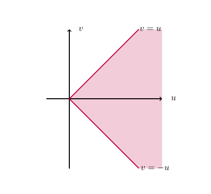
   $$\begin{eqnarray*} f_{U,V}(u,v) &=& f_{X,Y}(x(u,v),y(u,v))|J(u,v)| \\ &=& \begin{cases} \frac{1}{2} \lambda^2e^{-\lambda u} & \text{if } u+v > 0, u-v > 0, \\ 0 & \text{otherwise} \end{cases} \\ &=& \begin{cases} \frac{1}{2} \lambda^2e^{-\lambda u} & \text{if } u > 0,-u < v < u, \\ 0 & \text{otherwise.} \end{cases} \end{eqnarray*}$$ The region over which $f_{U,V}(u,v)>0$ is shown below.
   
2. The marginal pdf’s of $U$ and $V$ are respectively
   $$\begin{eqnarray*} f_U(u) &=& \int_{-\infty}^\infty f_{U,V}(u,v) dv = \begin{cases} \int_{-u}^u{1\over2} \lambda^2e^{-\lambda u} dv = \lambda^2u e^{-\lambda u} & \text{if }u>0,\\ 0 & \text{otherwise;} \end{cases} \\ f_V(v) &=& \int_{-\infty}^\infty f_{U,V}(u,v) du = \int_{|v|}^\infty \frac{1}{2} \lambda^2e^{-\lambda u}du = \frac{1}{2} \lambda e^{-\lambda|v|}, \qquad v\in{\mathbb R}. \end{eqnarray*}$$ Note that again we have $U =X+Y$ is the sum of two independent ${\rm Exp}(\lambda)$ random variables, so $U \sim {\rm Gamma} (2, \lambda)$.
   
3. Clearly, $f_{U,V}(u,v)=f_U(u) f_V(v)$ does not hold for all $u,v \in {\mathbb R}$, so $U$ and $V$ are not independent.