Chapter 16 Introduction to Linear Models

16.1 Introduction

In this section we present an introduction to Linear Models. Linear Models are the most common type of statistical model and is a wider class of model than is perhaps apparent at first. In Section 16.2, we introduce the concept of constructing a statistical model. In Section 16.3 we identify the key (linear) elements for a Linear Model and in Section 16.4 introduce the Normal (Gaussian) linear model. In Section 16.5 we define residuals the differences between the observations and what we expect to observe given the model. In Section 16.6 we consider least squares estimation for the parameters of linear models and show that for the Normal (Gaussian) linear model that this is equivalent to maximum likelihood estimation. In Section 16.7 we study two examples and consider how the residuals of the model can help us assess the appropriateness of the model. In Section 16.8 we briefly consider using the linear model for prediction which is one of the main purposes for constructing linear modeals. Finally in Section 16.9 we introduce the concept of nested models where a simpler model is nested within (a special case of) a more complex model. Whether to choose a simple or more complex model is a challenging statistical question and in this section we begin to study some of the considerations needed in making our choice.

16.2 Statistical models

One of the tasks of a statistician is the analysis of data. Statistical analysis usually involves one or more of the following:

• Summarising data;
  
• Estimation;
  
• Inference;
  
• Prediction.

In general, we statistically model the relationship between two or more random variables by considering models of the form: $$Y = f(\mathbf{X},\mathbf{\beta})+\epsilon,$$ where,

• $Y$ is the response variable;
  
• $f$ is some mathematical function;
  
• $\mathbf{X}$ is some matrix of predictor (input) variables;
  
• $\mathbf{\beta}$ are the model parameters;
  
• $\epsilon$ is the random error term (residual).

If we assume that $E[\epsilon]=0$, then $E[Y] = f(\mathbf{X},\mathbf{\beta})$ if $\mathbf{X}$ is assumed to be non-random. Otherwise $E[Y|\mathbf{X}] = f(\mathbf{X},\mathbf{\beta})$.

Consider the following examples where such modelling theory could be applied.

Cars on an intersection

We observe the number of cars passing an intersection over a one minute interval. We want to estimate the average rate at which cars pass this intersection.

If $Y$ is the number of cars passing the intersection over a one minute interval, then $Y$ is likely to have a Poisson distribution with mean $\lambda$. We want to estimate $\lambda$, the model parameter.

Industrial producivity

In economics, the production of an industry, $Y$, is modelled to be a function of the amount of labour available, $L$, and the capital input, $K$. In particular, the Cobb-Douglas Production Function is given to be $Y = C_0 L^\alpha K^\beta$.

Furthermore if $\alpha + \beta = 1$, then an industry is said to operate under constant returns to scale, that is, if capital and labour increase by a factor of $t$, then production also increases by a factor of $t$.

As a consultant to an economic researcher, you collect production, labour and capital data for a specific industry and want to estimate the functional relationship and test whether $\alpha + \beta = 1$ in this industry. The problem will have the following components:

• A theoretical model: $Y = C_0 L^\alpha K^\beta$;
  
• A statistical model: $\log Y = C^\ast + \alpha \log L + \beta \log K + \epsilon$;
  
• Some estimations: $C^\ast$, $\alpha$ and $\beta$;
  
• A test: does $\alpha + \beta = 1$?
  

Blood pressure

Suppose we are interested in studying what factors affect a person’s blood pressure. We have a proposed statistical model, where blood pressure depends on a large number of factors:

$$\text{Blood pressure} = f \left( \begin{array}{c c c} \text{age}, & \text{weight}, & \text{gender}, \\ \text{activity level}, & \text{personality type}, & \text{time of day}, \\ & \text{genetic predisposition} & \end{array} \right) + \epsilon.$$

We want to estimate the functional relationship $f$ and potentially test which of the factors has a significant influence on a person’s blood pressure.

16.3 The linear model

Suppose that $Y_1, Y_2, \ldots Y_n$ are a collection of response variables, with $Y_i$ dependent on the predictor variables $\mathbf{X}_i = \begin{pmatrix} 1 & X_{1,i} & \cdots & X_{p,i} \end{pmatrix}$. Assume that, for $i=1,2,\ldots, n$,
$$Y_i = f(\mathbf{X}_i,\mathbf{\beta}) + \epsilon_i = \beta_0 + \beta_1X_{1i} + \dots + \beta_p X_{pi} + \epsilon_i.$$ A matrix representation of the model is $\mathbf{Y} = \mathbf{Z} \mathbf{\beta} + \mathbf{\epsilon}$, where
$$\begin{eqnarray*} \mathbf{Y} = \left[ \begin{array}{c} Y_1 \\ Y_2 \\ \vdots \\ Y_n \end{array} \right], &\qquad \qquad \qquad& \mathbf{Z} = \left[ \begin{array}{cccc} 1 & X_{11} & \cdots & X_{p1} \\ 1 & X_{12} & \cdots & X_{p2} \\ \vdots & \vdots & \ddots & \vdots \\ 1 & X_{1n} & \cdots & X_{pn} \end{array} \right], \\ \mathbf{\beta} = \left[ \begin{array}{c} \beta_0 \\ \beta_1 \\ \vdots \\ \beta_p \end{array} \right], &\quad \qquad \qquad& \mathbf{\epsilon} = \left[ \begin{array}{c} \epsilon_1 \\ \epsilon_2 \\ \vdots \\ \epsilon_n \end{array} \right]. \end{eqnarray*}$$

Here $\mathbf{Z}$ is called the design matrix and in models with a constant term includes a column of ones as well as the data matrix $\mathbf{X}$ and possibly functions of $\mathbf{X}$. If no constant or functions are included in the model, $\mathbf{Z}$ and $\mathbf{X}$ are equivalent.

It is common to represent linear models in matrix form. As we shall observe in Section 17 using matrices allows for concise representations of key quantities such as parameter estimates and calculating residuals. Familiarity with core concepts from linear algebra is essential in understanding and manipulating linear models.

Linear Model

A model is considered to be linear if it is linear in its parameters.

Consider the following models, and why they are linear/non-linear:

• $Y_i = \beta_0 + \beta_1 X_{1i} + \beta_2 X_{2i} + \epsilon_i$ is linear;
  
• $Y_i = \beta_0 + \beta_1 X_{1i} + \beta_2 X_{2i}^2 + \epsilon_i$ is linear;
  
• $\log Y = \log C_0 L^\alpha K^\beta + \epsilon$ is considered linear since we can transform the model into $\log Y = C_0 + \alpha \log L + \beta \log K + \epsilon$;
  
• $Y = \frac{\beta_1}{\beta_1 - \beta_2} \left[ e^{-\beta_2 X} - e^{\beta_1 X} \right] + \epsilon$ is non-linear.

A linear model therefore has the following underlying assumptions:

• The model form can be written $Y_i = \beta_0 + \beta_1 X_{1i} + \cdots + \beta_p X_{pi} + \epsilon_i$ for all $i$;
  
• $E[\epsilon_i]=0$ for all $i$;
  
• $\text{Var}(\epsilon_i) = \sigma^2$ for all $i$;
  
• $\text{Cov}(\epsilon_i, \epsilon_j) = 0$ for all $i \ne j$.

16.4 The Normal (Gaussian) linear model

Normal Linear Model

A normal linear model assumes:

• A model form given by $Y_i = \beta_0 + \beta_1 X_{1i} + \cdots + \beta_p X_{pi} + \epsilon_i$ for all $i$;
  
• $\epsilon_i \sim N(0,\sigma^2)$ are independent and identically distributed (i.i.d.).
  

There are two key implications of these assumptions:

• $Y_i \sim N(\beta_0 + \beta_1 X_{1i} + \cdots + \beta_p X_{pi},\sigma^2)$ for all $i=1,\dots,n$. Equivalently writing this in matrix form, $\mathbf{Y} \sim N_n \left( \mathbf{Z} \mathbf{\beta}, \sigma^2 \mathbf{I}_n \right)$ where $N_n$ is the $n$-dimensional multivariate normal distribution. Note that if two random variables $X$ and $Y$ are normally distributed, then $\text{Cov}(X,Y)=0$ if and only if $X$ and $Y$ are independent.
  
• Since $\text{Cov}(\epsilon_i,\epsilon_j)=0$ for all $i \ne j$, then $\text{Cov}(Y_i,Y_j)=0$ for all $i \ne j$, and $Y_1, Y_2,\dots,Y_n$ are independent. (Remember that for Normal (Gaussian) random variables $X$ and $Y$ are independent if and only if they are uncorrelated $Cov (X,Y) =0$, see Section 15.2.)

16.5 Residuals

We have the statistical model: $$Y = f (\mathbf{X},\beta) + \epsilon,$$ which satisfies $E[\epsilon] =0$, and hence, $E[Y]=f(\mathbf{X},\beta)$. The above equation can be rewritten as $$\epsilon = Y - f (\mathbf{X},\beta).$$ Suppose that we have observed responses $y_1, y_2, \ldots, y_n$, where observation $i$ has predictors $\mathbf{x}_i$. Then given parameters $\beta$, the expected value for the $i^{th}$ response is $f (\mathbf{x}_i,\beta)$, and is often denoted $\hat{y}_i$. The residual $\epsilon_i$ is the difference between the observed response and its expected value:
$$\epsilon_i = y_i - \hat{y}_i = y_i - f (\mathbf{x}_i,\beta).$$ Note that if $f(\mathbf{x}_i, \beta) = \alpha + \beta x_i$, then
$$\epsilon_i = y_i - \{ \alpha + \beta x_i \}.$$

An assumption of the Normal linear model is that $\epsilon_i \sim N(0,\sigma^2)$, independent of the value of $f(x_i, \beta) = \alpha +\beta x_i$. Therefore plotting residual values against expected values is one way of testing the appropriateness of the model.

16.6 Straight Line, Horizontal Line and Quadratic Models

In this section we look at three types of linear model that we might choose to assume to fit some data $X_i$ and $Y_i$. Making this choice appropriately is a key part of the statistical analysis process.

Straight line model

The straight line model is the simple linear regression model given by

$$y_{i} = \alpha + \beta x_i + \epsilon_i, \qquad \text{for all } i =1,\ldots n.$$

Given a straight line model, we have $E[Y] = \alpha + \beta X$. The key part of using a straight line model is to estimate the values of $\alpha$ and $\beta$.

Let $\hat{\alpha}$ and $\hat{\beta}$ be the estimated values of $\alpha$ and $\beta$, respectively. We call $y_i$ the $i^{th}$ observed value and $\hat{y}_i = \hat{\alpha} + \hat{\beta} x_i$ the $i^{th}$ fitted value (expected value).

Model deviance

$D = \sum_{i=1}^{n} \left(y_{i}-\hat{y}_i\right)^{2}$ is called the model deviance.

Since $\epsilon_i = y_{i}-\hat{y}_i$, the model deviance is the sum of the squares of the residuals, $$D = \sum_{i=1}^n \epsilon_i^2.$$

For the estimated line to fit the data well, one wants an estimator of $\alpha$ and $\beta$ that minimises the model deviance. So, choose $\hat{\alpha}$ and $\hat{\beta}$ to minimise $$D = \sum\limits_{i=1}^{n} \left(y_{i}-\hat{y}_i\right)^{2} = \sum\limits_{i=1}^n \left( y_i-\alpha-\beta x_i \right)^2.$$ To minimise $D$ we calculate the stationary points of $D$, that is, the values of $\alpha$ and $\beta$ for which the two first order partial derivatives vanish.
$$\begin{align*} \frac{\partial D}{\partial \alpha} &= -2 \sum\limits_{i=1}^n \left(y_i- \left( \hat{\alpha} + \hat{\beta}x_i \right) \right) = 0 \\[3pt] \frac{\partial D}{\partial \beta} &= -2 \sum\limits_{i=1}^n x_i \left(y_i - \left( \hat{\alpha} + \hat{\beta} x_i \right) \right) = 0 \end{align*}$$ Solving these equations simultaneously gives
$$\begin{align*} \hat{\beta} &= \frac{ \sum\limits_{i=1}^n \left( x_i-\bar{x} \right) \left( y_i-\bar{y} \right) }{ \sum\limits_{i=1}^n \left( x_i-\bar{x} \right)^2} = \frac{(n-1)s_{xy}}{(n-1)s_x^2} = \frac{s_{xy}}{s_x^2}, \\[3pt] \hat{\alpha} &= \bar{y} - \hat{\beta}\bar{x}. \end{align*}$$

Note that $\hat{\alpha}$ and $\hat{\beta}$ are called least squares estimators of $\alpha$ and $\beta$. We did not use the normality assumption in our derivation, so the least squares estimators are invariant to the choice of distribution for the error terms.

If we include the assumption of normality, then it can be shown that $\hat{\alpha}$ and $\hat{\beta}$ are also the MLEs of $\alpha$ and $\beta$ respectively.

Let $y_1, y_2, \ldots, y_n$ be observations from a normal linear model:
$$y= \alpha + \beta x + \epsilon,$$ where $\epsilon \sim N(0,\sigma^2)$ and $x_1,x_2, \ldots, x_n$ are the predictor variables. Then
$$\hat{\beta} = \frac{s_{xy}}{s_x^2} \qquad \qquad \mbox{and} \qquad \qquad \hat{\alpha} = \bar{y} - \hat{\beta}\bar{x},$$

are the maximum likelihood estimates of $\beta$ and $\alpha$, respectively.

First, note that
$$y_i \sim N (\alpha + \beta x_i, \sigma^2).$$ Therefore the likelihood is given by
$$\begin{eqnarray*} L (\alpha,\beta, \sigma^2) &=& \prod_{i=1}^n f(y_i | \alpha, \beta, x_i, \sigma^2) \\ &=& \prod_{i=1}^n \frac{1}{\sqrt{2 \pi \sigma^2}} \exp \left( - \frac{1}{2 \sigma^2} \left\{ y_i - (\alpha +\beta x_i) \right\}^2 \right) \\ &=& (2 \pi \sigma^2)^{-\frac{n}{2}} \exp \left( -\frac{1}{2 \sigma^2} \sum_{i=1}^n \left\{ y_i - (\alpha +\beta x_i) \right\}^2 \right). \end{eqnarray*}$$ The log-likelihood is
$$l (\alpha,\beta, \sigma^2) = - \frac{n}{2} \log \left(2 \pi \sigma^2 \right) -\frac{1}{2 \sigma^2} \sum_{i=1}^n \left\{ y_i - (\alpha +\beta x_i) \right\}^2.$$

In order to maximise the log-likelihood with respect to $\alpha$ and $\beta$, we note that:

• $- \frac{n}{2} \log \left(2 \pi \sigma^2 \right)$ does not involve $\alpha$ and $\beta$, so can be treated as a constant;
  
• Since $\sigma^2 >0$, $-\frac{1}{2 \sigma^2} \sum_{i=1}^n \left\{ y_i - (\alpha +\beta x_i) \right\}^2$ will reach its maximum when $\sum_{i=1}^n \left\{ y_i - (\alpha +\beta x_i) \right\}^2$ is minimised.

Therefore the parameter values $\hat{\alpha}$ and $\hat{\beta}$ which maximise $l (\alpha,\beta, \sigma^2)$ are the parameter values which minimise $\sum_{i=1}^n \left\{ y_i - (\alpha +\beta x_i) \right\}^2$, i.e. the least squares estimates.

Note that the maximum likelihood estimates of $\hat{\alpha}$ and $\hat{\beta}$ do not depend on the value of $\sigma^2$.

Horizontal line model

The horizontal line model is the simple linear regression model given by

$$y_i = \mu + \epsilon_i, \qquad \text{for } i=1,\dots,n.$$

Given a horizontal line model, we have $E[Y]=\mu$. Specifically in this model, we assume the predictor variable has no ability to explain the variance in the response variable.

To estimate $\mu$ by least squares we minimise $D = \sum\limits_{i=1}^n (y_i - \mu)^2$. Setting $\frac{\partial D}{\partial \mu} = 0$ and solving, we get $\hat{\mu} = \bar{y}$.

Let $D_1$ be the deviance of the straight line model and $D_2$ be the deviance of the horizontal line model. The straight line model does a better job of explaining the variance in $Y$ if $D_1 \leq D_2$, in which case we say that the straight line model fits the data better.

Quadratic line model

The quadratic model is the simple linear regression model given by

$$y_i = \alpha + \beta x_i + \gamma x_i^2 + \epsilon_i, \qquad \text{for } i=1,\dots,n.$$

To estimate $\alpha$, $\beta$ and $\gamma$ by least squares we minimise
$$D = \sum\limits_{i=1}^n \left( y_i - (\alpha + \beta x_i + \gamma x_i^2) \right)^2.$$

If we let $D_3 = \sum\limits_{i=1}^n \left( y_i - (\hat{\alpha} + \hat{\beta} x_i + \hat{\gamma} x_i^2) \right)^2$ be the model deviance, then the quadratic model fits the data better than the straight line model if $D_3 \leq D_1$.

16.7 Examples

Tyre experiment

A laboratory tests tyres for tread wear by conducting an experiment where tyres from a particular manufacturer are mounted on a car. The tyres are rotated from wheel to wheel every 1000 miles, and the groove depth is measured in mils (0.001 inches) initially and after every 4000 miles giving the following data (Tamhane and Dunlap, 2000):

Mileage (1000 miles)	Groove Depth (mils)
0	394.23
4	329.50
8	291.00
12	255.17
16	229.33
20	204.83
24	179.00
28	163.83
32	150.33

Watch Video 24 for a work through fitting linear models to the tyre experiment in R and a discussion of choosing the most appropriate linear model. A work through of the analysis is presented below.

Video 24: Tyre Experiment

Firstly we have to determine which is the response variable and which is the predictor (or controlled) variable. Secondly, we have to hypothesise a functional relationship between the two variables, using either theoretical relationships or exploratory data analysis.

Let the response variable, $Y$, be groove depth and let the predictor variable, $X$, be mileage. Consider a plot of mileage vs. depth:

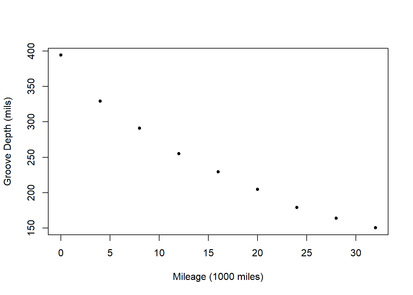
Note that as mileage increases, the groove depth decreases.

The straight line model for the data is

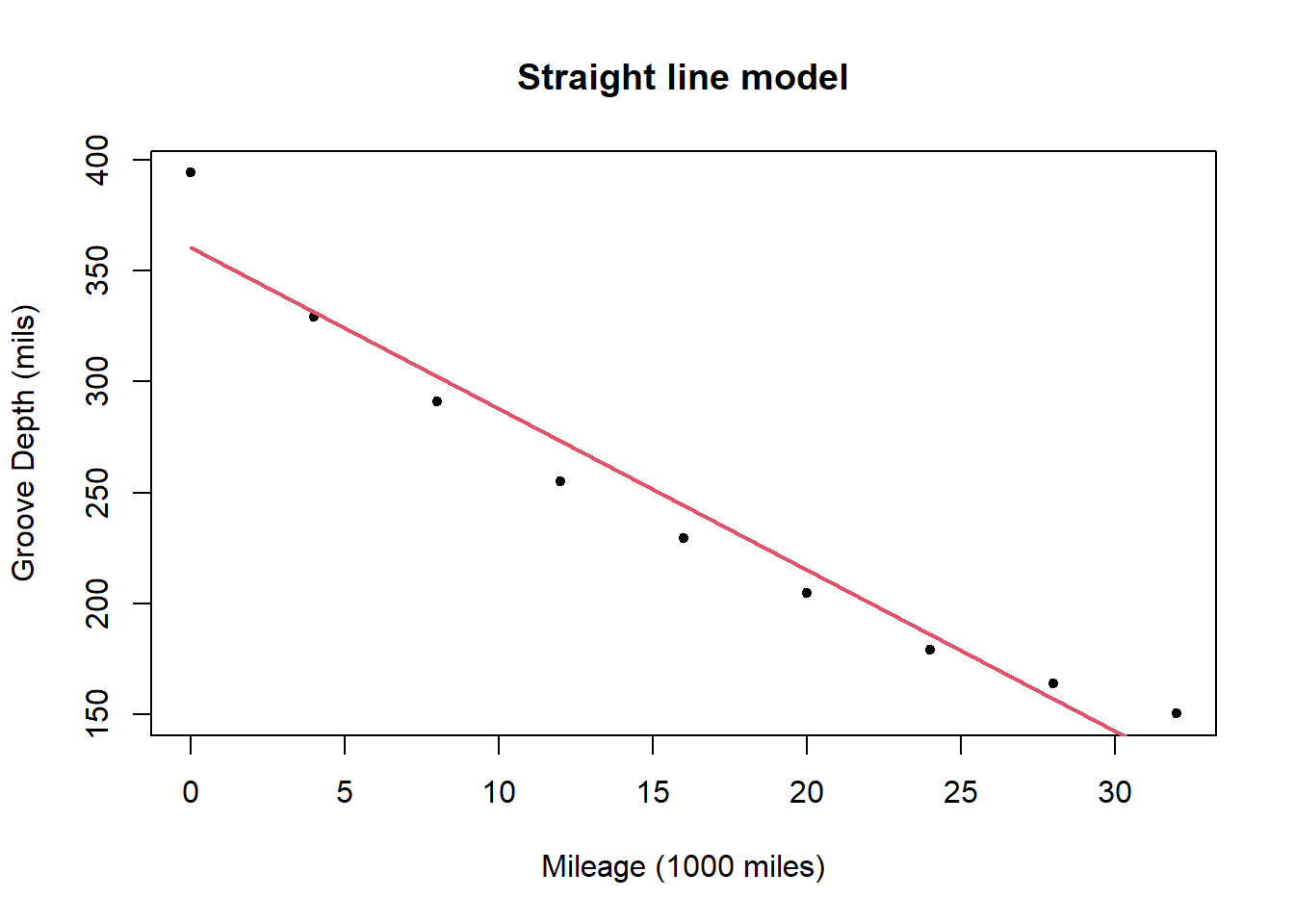
The straight line model is:
$$y= 360.599 -7.279 x + \epsilon$$

and the deviance for the model is 2524.8.

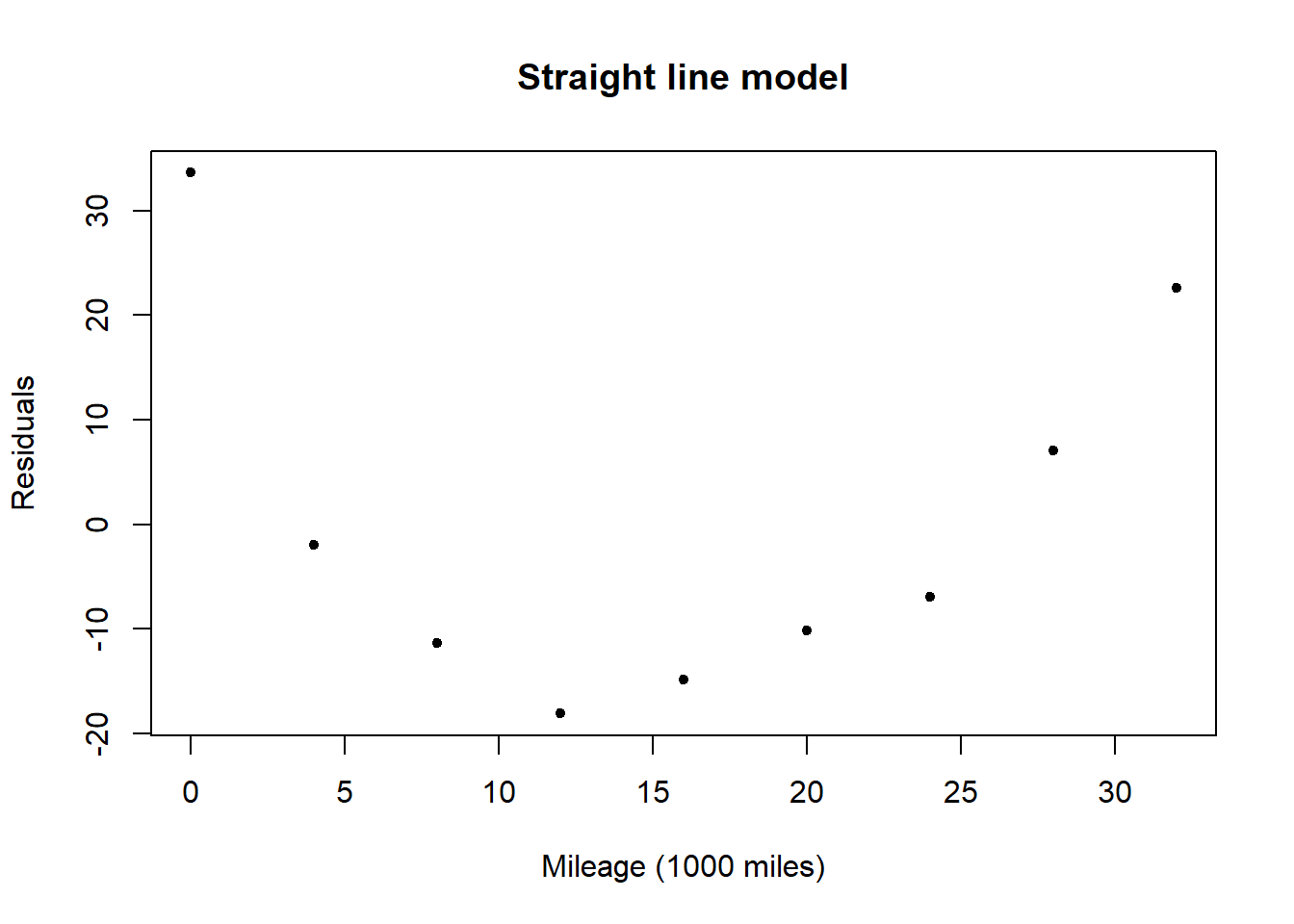
A plot of the residuals for the straight line model shows a relationship with $x$ (mileage), possibly quadratic. This informs us that there is a relationship between mileage and groove depth which is not captured by the linear model.

The horizontal line model for the data is

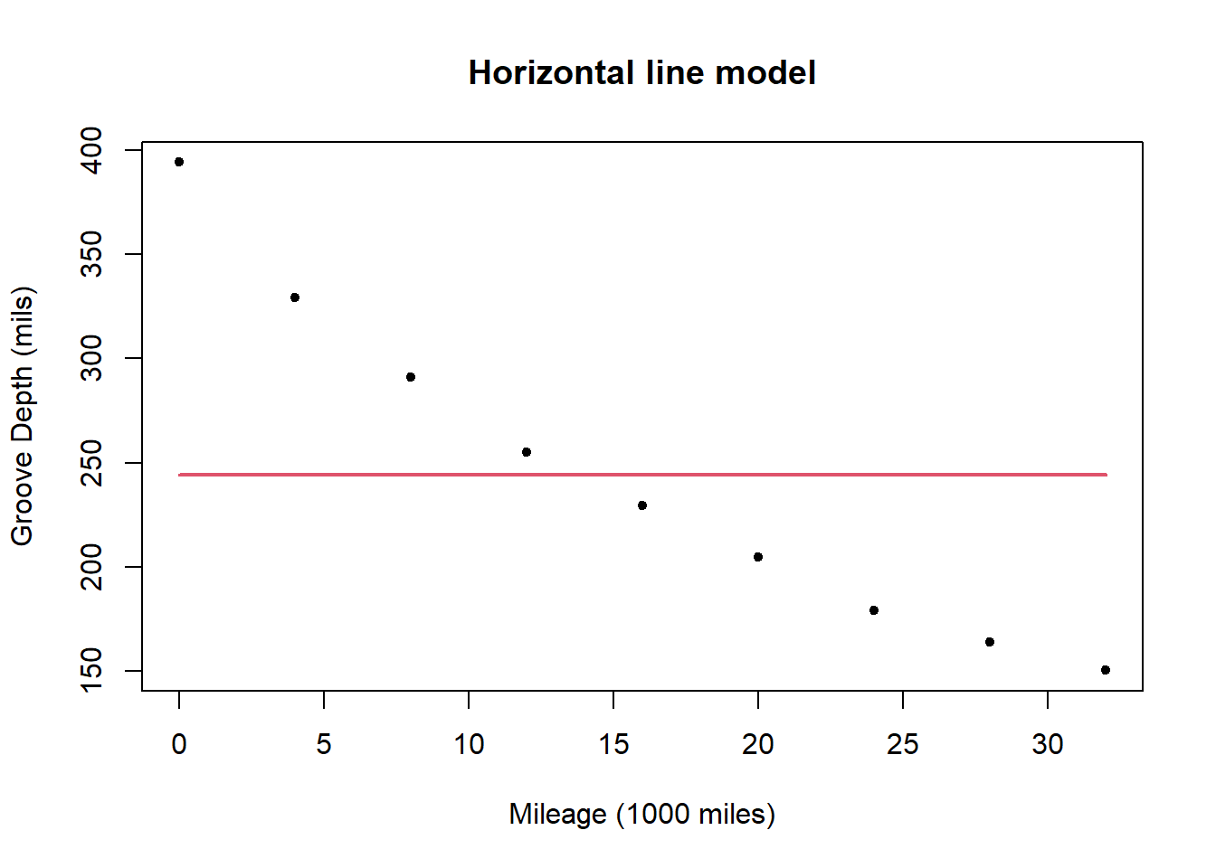
The horizontal line model is: $$y= 244.136 + \epsilon.$$

The deviance for the model is 53388.7, which is much higher than the deviance for the straight line model suggesting it is a considerably worse fit to the data. In this case the poorness of the fit of the horizontal line model is obvious, but later will explore ways of making rigorous the comparison between models.

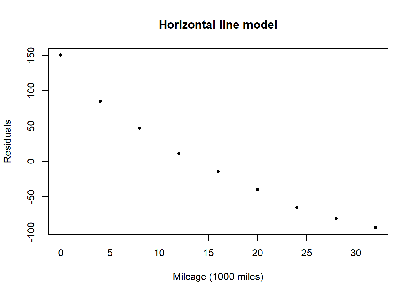
A plot of the residuals for the horizontal line model shows a very clear downward trend with $x$ (mileage) confirming that the horizontal line model does not capture the relationship between mileage and groove depth.

The quadratic model for the data is

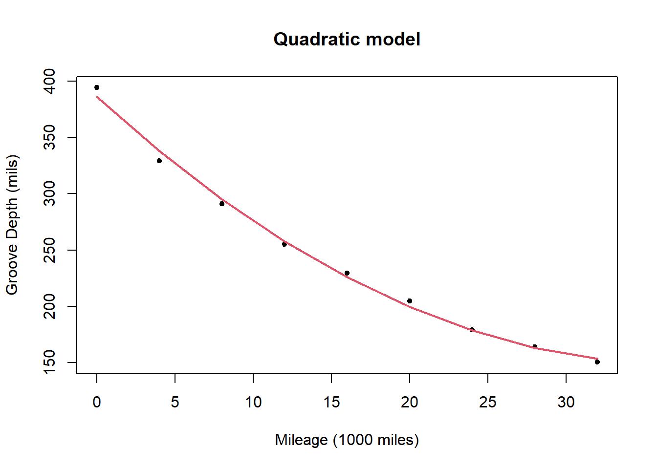
The quadratic model is $$y= 386.199 -12.765 x + 0.171 x^2 + \epsilon$$ and the deviance for the model is 207.65. This is a substantial reduction on the deviance of the straight line model suggesting that it offers a substantial improvement.

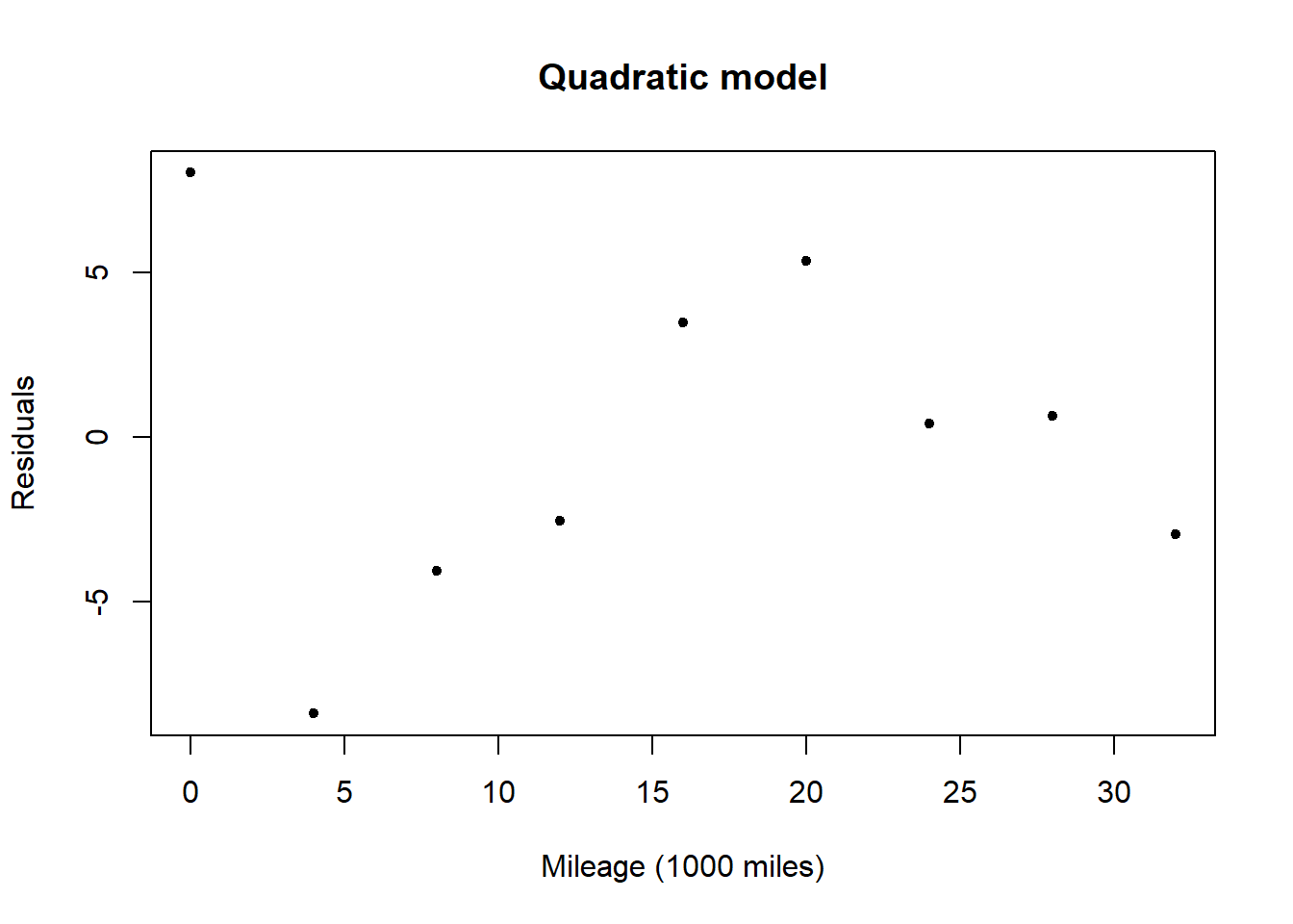
A plot of the residuals for the quadratic model shows no obvious pattern. This suggests that the model could be appropriate in capturing the relationship between mileage and groove depth, with the differences between observed and expected values due to randomness.

Drug effectiveness

Suppose we are interested in the effect a certain drug has on the weight of an organ. An experiment is designed in which rats are randomly assigned to different treatment groups in which each group contains $J$ rats and receives the drug at one of 7 distinct levels. Upon completion of the treatment, the organs are harvested from the rats and weighed.

Let $Y_{ij}$ be the weight of the organ (response variable) of the $j^{th}$ rat in the $i^{th}$ treatment,
$$Y_{ij} = \mu_i + \epsilon_{ij}, \qquad \text{for all } i=1,\dots,7 \text{ and } j=1,\dots,J.$$

The model is linear in the parameters $\mu_1, \mu_2,\dots,\mu_7$. Specifically our aim is to test whether $\mu_1 = \mu_2 = \cdots = \mu_7$. Estimating using least squares minimises $$D = \sum\limits_{i=1}^7 \sum\limits_{j=1}^J (y_{ij} - \mu_i)^2,$$

and least squares estimators are given by: $$\hat{\mu}_i = \bar{y}_{i.} = \frac{1}{J} \sum\limits_{i=1}^J y_{ij}.$$

The estimate of the mean for level $i$ is the sample mean of the $J$ rats receiving treatment level $i$.

16.8 Prediction

A linear model identifies a relationship between the response variable $y$ and the predictor variable(s), $\mathbf{x}$. We can then use the linear model to predict $y^\ast$ given predictor variables $\mathbf{x}^\ast$.

Given the model, $$Y = f (\mathbf{x},\beta) + \epsilon$$ where $E[\epsilon]=0$, we have that our best estimate of $y^\ast$ given $\mathbf{x}^\ast$ and model parameters $\hat{\beta}$ is
$$y^\ast = E[Y | \mathbf{x}^\ast, \hat{\beta}]= f(\mathbf{x}^\ast, \hat{\beta}) = \hat{\beta}_0 + \sum_{j=1}^p \hat{\beta}_j x_j^\ast.$$

We will discuss later the uncertainty in the prediction of $y^\ast$ which depends upon the variance of $\epsilon$, uncertainty in the estimation of $\hat{\beta}$ and how far the $x_j^\ast$s are from the mean of the $x_j$s.

For Example 16.7.1 (Tyre experiment), we can use the three models (straight line, horizontal line, quadratic) to predict the groove depth (mils) of the tyres after 18,000 miles. The predicted values are:

• Straight line model - $y^\ast = 360.599 -7.279 (18) = 229.577$.
  
• Horizontal line model - $y^\ast = 244.136$.
  
• Quadratic model - $y^\ast = 386.199 -12.765 (18) + 0.171 (18^2) = 211.833$.

16.9 Nested Models

In Example 16.7.1 (Tyre experiment), we considered three models:

• Straight line model: $y = \alpha + \beta x + \epsilon$.
  
• Horizontal line model: $y = \mu + \epsilon$.
  
• Quadratic model: $y = \alpha + \beta x + \gamma x^2+ \epsilon$.

The quadratic model is the most general of the three models. We note that if $\gamma =0$, then the quadratic model reduces to the straight line model. Similarly letting $\beta= \gamma =0$ in the quadratic model and with $\mu = \alpha$, the quadratic model reduces to the horizontal model. That is, the horizontal line and straight line models are special cases of the quadratic model, and we say that the horizontal line and straight line models are nested models in the quadratic model. Similarly the horizontal line model is a nested model in the straight line model.

Nested model

Model $A$ is a nested model of Model $B$ if the parameters of Model $A$ are a subset of the parameters of Model $B$.

Let $D_A$ and $D_B$ denote the deviances of Models $A$ and $B$, respectively. Then if Model $A$ is a nested model of Model $B$, $$D_B \leq D_A.$$

That is, the more complex model with additional parameters will fit the data better.

Let $\alpha = (\alpha_1, \alpha_2, \ldots, \alpha_K)$ denote the $K$ parameters of Model $A$ and let $\beta = (\alpha_1, \alpha_2, \ldots, \alpha_K,\delta_1, \ldots, \delta_M)$ denote the $K+M$ parameters of Model $B$.

If $\hat{\alpha} = (\hat{\alpha}_1, \hat{\alpha}_2, \ldots, \hat{\alpha}_K)$ minimise the deviance under Model $A$, then the parameters $(\hat{\alpha}_1, \hat{\alpha}_2, \ldots, \hat{\alpha}_K,0, \ldots, 0)$, where $\delta_i =0$ will achieve the deviance $D_A$ under Model $B$. Thus $D_B$ can be at most equal to $D_A$.

Since more complex models will better fit data (smaller deviance), why not choose the most complex model possible?

There are many reasons and these include interpretability, can you interpret the relation between $x_i$ and $y_i$ (for example, the time taken to run 100 metres is unlikely to be a good predictor for performance on a maths test) and predictive power, given a new predictor observation $x^\ast$ can we predict $y^\ast$.

Student Exercise

Attempt the exercise below.

Given the following theoretical relationships between $Y$ and $X$, with $\alpha$ and $\beta$ unknown, can you find ways of expressing the relationship in a linear manner?

1. $Y = \alpha e^{\beta X}$,
   
2. $Y = \alpha X^{\beta}$,
   
3. $Y = \log(\alpha+e^{\beta X})$.
   

Solution to Exercise 16.1.

1. Take logs, so $\log Y = \log \alpha + \beta X$. Hence, $Y' = \alpha' + \beta X$ where $Y' = \log Y, \alpha' = \log \alpha$.
   
2. Again, take logs, so $\log Y = \log \alpha + \beta \log X$. Hence, $Y' = \alpha' + \beta X'$ where $Y' = \log Y$, $\alpha' = \log \alpha$, $X' = \log X$.
   
3. This cannot be written as a linear model.