Chapter 13 Expectation, Covariance and Correlation

In this section, we study further properties of expectations of random variables. We move on from the expectation of a single random variable to consider the expectation of the function of a collection of random variables, $X_1, X_2, \ldots, X_n$. We pay particular attention to the expectation of functions of two random variables $X$ and $Y$, say. We define the covariance as a measure of how the random variables $X$ and $Y$ vary together and the correlation which provides a measure of linear dependence between two random variables $X$ and $Y$.

13.1 Expectation of a function of random variables

If $X_1,X_2,\dots,X_n$ are jointly continuous, then the expectation of the function $g(X_1,X_2,\dots,X_n)$ is given by
$$E[g(X_1,\dots,X_n)] = \int\cdots\int_{\mathbb{R}^n} g(x_1,\dots,x_n) f_{X_1,\dots,X_n}(x_1,\dots,x_n) \,dx_1 \cdots \,dx_n$$

Note that if $X_1,X_2,\dots,X_n$ are discrete, we replace the integrals by summations and the joint p.d.f. with the joint p.m.f.

Expectation has the following important properties:

• The expectation of a sum is equal to the sum of the expectations (see Section 5.3):
  $$E \left[ \sum\limits_{i=1}^{n} X_i \right] = \sum\limits_{i=1}^{n} E[X_i];$$
• If $X$ and $Y$ are independent, then
  $$E[XY] = E[X]E[Y];$$
• If $X$ and $Y$ are independent and $g$ and $h$ are any real functions, then
  $$E[g(X)h(Y)]=E[g(X)]E[h(Y)].$$

13.2 Covariance

Covariance

The covariance of two random variables, $X$ and $Y$, is defined by
$$\text{Cov}(X,Y) = E\left[(X-E[X])(Y-E[Y])\right]$$

Covariance has the following important properties:

• Covariance is equal to the expected value of the product minus the product of the expected values.
  $$\text{Cov} (X,Y) = E[XY]-E[X]E[Y].$$
• If $X$ and $Y$ are independent, then $cov(X,Y)$ = 0. The converse is NOT true.
  
• The covariance of two equal random variables is equal to the variance of that random variable.
  $$\text{Cov}(X,X) = \text{Var}(X).$$
• The covariance of a scalar multiple of a random variable (in either argument) is equal to the scalar multiple of the covariance. Additionally covariance is invariant under the addition of a constant in either argument.
  $$\text{Cov} (aX+b,cY+d) = ac \text{Cov}(X,Y).$$
• The covariance of a linear combination of random variables is equal to a linear combination of the covariances.
  $$\text{Cov} \left( \sum_{i=1}^m a_iX_i, \sum_{j=1}^n b_jY_j \right) = \sum_{i=1}^m \sum_{j=1}^n a_ib_j \text{Cov}(X_i,Y_j).$$
• There is a further relationship between variance and covariance:
  $$\text{Var}(X+Y) = \text{Var}(X) + \text{Var}(Y) + 2\text{Cov}(X,Y).$$
• More generally this relationship between variance and covariance becomes:
  $$\text{Var} \left( \sum_{i=1}^n a_iX_i \right) = \sum_{i=1}^n a_i^2 \text{Var}(X_i) + 2 \sum_{1 \leq i < j \leq n} a_ia_j\text{Cov}(X_i,X_j).$$
• Consider the above identity if $X_1,X_2,\dots,X_n$ are independent, and each $a_i$ is equal to $1$ (see Section 5.3). Then we have:
  $$\text{Var} \left( \sum_{i=1}^n X_i \right) = \sum_{i=1}^n \text{Var} (X_i).$$

Density on a circle

Suppose that $X$ and $Y$ have joint probability density function $$f_{X,Y} (x,y) = \left\{ \begin{array}{ll} \frac{1}{\pi} \qquad \qquad & x^2 + y^2 \leq 1 \\ 0 & \mbox{otherwise}. \end{array} \right.$$

Then $\text{Cov} (X,Y) =0$ but $X$ and $Y$ are not independent.

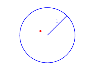
Figure 13.1: Example: Point at $(x,y) =(-0.25,0.15)$.

Watch Video 21 for an explanation of Example 13.2.2: Density on a circle or see the written explanation below.

Video 21: Density on a circle

Explanation - Example 13.2.2: Density on a circle.

We begin by computing $E[X]$, $E[Y]$ and $E[XY]$.
To compute $E[X]$, we first find $f_X (x)$.
Note that if $X=x$, then
$$x^2 + y^2 \leq 1 \hspace{1cm} \Leftrightarrow \hspace{1cm} y^2 \leq 1-x^2 \hspace{1cm} \Leftrightarrow \hspace{1cm} - \sqrt{1-x^2} \leq y \leq \sqrt{1-x^2}.$$ Hence, for $-1 < x< 1$,
$$\begin{eqnarray*} f_X (x) &=& \int_{-\sqrt{1-x^2}}^{\sqrt{1-x^2}} f_{X,Y} (x,y) \, dy \\ &=& \int_{-\sqrt{1-x^2}}^{\sqrt{1-x^2}} \frac{1}{\pi} \, dy \\ &=& \left[ \frac{y}{\pi} \right]_{-\sqrt{1-x^2}}^{\sqrt{1-x^2}} \\ &=& \frac{\sqrt{1-x^2}}{\pi} - \frac{-\sqrt{1-x^2}}{\pi} = \frac{2 \sqrt{1- x^2}}{\pi}. \end{eqnarray*}$$ Thus
$$f_X (x) = \left\{ \begin{array}{ll} \frac{2 \sqrt{1- x^2}}{\pi} \qquad \qquad & -1 < x < 1 \\ 0 & \mbox{otherwise}. \end{array} \right.$$ see Figure 13.2.

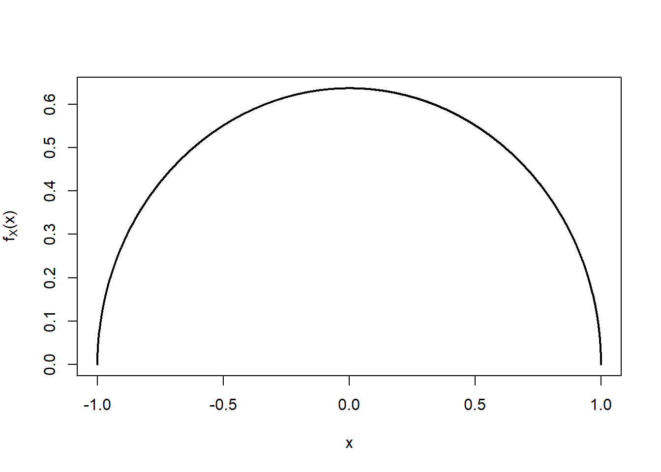
Figure 13.2: Plot of the p.d.f. of $X$.

Therefore $E[X]$ is given by
$$\begin{eqnarray*} E[X] &=& \int_{-\infty}^\infty x f_X (x) \, dx \\ &=& \int_{-1}^1 x \frac{2 \sqrt{1- x^2}}{\pi} \, dx \\ &=& \int_{-1}^0 x \frac{2 \sqrt{1- x^2}}{\pi} \, dx + \int_0^1 x \frac{2 \sqrt{1- x^2}}{\pi} \, dx \end{eqnarray*}$$ Using a change of variable $v=-x$ in the first integral:
$$\begin{eqnarray*} \int_{-1}^0 x \frac{2 \sqrt{1- x^2}}{\pi} \, dx &=& \int_1^0 (-v) \frac{2 \sqrt{1- (-v)^2}}{\pi} \, (-dv) \\ &=& - \int_0^1 v \frac{2 \sqrt{1- (v)^2}}{\pi} \, dv. \end{eqnarray*}$$ Hence, the red and blue integrals below are equal:
$$\begin{eqnarray*} E[X] &=& - \color{red}{\int_0^1 v \frac{2 \sqrt{1- v^2}}{\pi} \, dv} + \color{blue}{\int_0^1 x \frac{2 \sqrt{1- x^2}}{\pi} \, dx} \nonumber \\ &=& 0. \end{eqnarray*}$$ A symmetry argument gives that
$$f_Y (y) = \left\{ \begin{array}{ll} \frac{2 \sqrt{1- y^2}}{\pi} \qquad \qquad & -1 < y < 1 \\ 0 & \mbox{otherwise}, \end{array} \right.$$ and $E[Y]=0$.
Now
$$\begin{eqnarray*} E[XY]&=& \int \int_{x^2+y^2 \leq 1} xy \frac{1}{\pi} \, dy \, dx \\ &=& \int_{-1}^1 \int_{-\sqrt{1-x^2}}^{\sqrt{1-x^2}} xy \frac{1}{\pi} \, dy \, dx \\ % Condition on the size of x, then y needs to be in the given range. &=& \int_{-1}^1 \frac{x}{\pi} \left[ \frac{y^2}{2} \right]_{-\sqrt{1-x^2}}^{\sqrt{1-x^2}} \, dx \\ &=& \int_{-1}^1 \frac{x}{2\pi} \left[ 1-x^2 - (1-x^2)\right] \, dx \\ &=& \int_{-1}^1 \frac{x}{2\pi} (0) \, dx =0. \end{eqnarray*}$$ Therefore
$$cov (X,Y) = E[XY] - E[X] E[Y] = 0 - 0\times 0 =0.$$ However, $X$ and $Y$ are not independent.
Note that for $x=0.8$ and $y=0.8$, $x^2 + y^2 = 0.8^2 + 0.8^2 = 1.28 >1$, so
$$f_{X,Y} (0.8,0.8) =0.$$ However, $f_X(0.8) = \frac{2}{\pi} \sqrt{1-0.8^2} = 0.382$ and also $f_Y(0.8)=0.382$ giving
$$f_X(0.8) f_Y(0.8) =0.382 \times 0.382 \neq 0 = f_{X,Y} (0.8,0.8).$$

13.3 Correlation

Correlation

If $\text{Var}(X)>0$ and $\text{Var}(Y)>0$, then the correlation of $X$ and $Y$ is defined by
$$\rho(X,Y) = \frac{\text{Cov}(X,Y)}{\sqrt{\text{Var}(X)\text{Var}(Y)}}.$$

Correlation has the following important properties:

• $-1 \leq \rho(X,Y) \leq 1$.
  
• If $X$ and $Y$ are independent, then $\rho(X,Y)=0$. Note, again, that the converse is not true.
  
• Correlation is invariant under a scalar multiple of a random variable (in either argument) up to a change of sign. Additionally correlation is invariant under the addition of a constant in either argument.
  $$\rho (aX+b,cY+d) = \begin{cases} \rho(X,Y), & \text{if } ac>0, \\[3pt] -\rho(X,Y), & \text{if } ac<0. \end{cases}$$

For example, the correlation between height and weight of individuals will not be effected by the choice of units of measurement for height (cm, mm, feet) and weight (kg, pounds, grammes) but the covariance (and variance) will change depending upon the choice of units.

Task: Session 7

Attempt the R Markdown file for Session 7:
Session 7: Joint distributions

Student Exercises

Attempt the exercises below.

Show that if $X$ and $Y$ are two independent random variables then $\text{Cov} (X,Y) =0$.

Solution to Exercise 13.1.

If $X$ and $Y$ are independent, then $E[XY] = E[X]E[Y]$, and therefore $$\text{Cov} (X,Y)= E[XY]- E[X]E[Y] = E[X]E[Y] - E[X]E[Y] =0.$$

Assume that $X$ and $Y$ are two random variables with $\text{Var}(X) = \text{Var}(Y) = \frac{11}{144}$ and $\text{Cov}(X,Y) = -\frac{1}{144}$. Find the variance of $\frac{1}{2} X + Y$.

Solution to Exercise 13.2.

$$\begin{eqnarray*} \text{Var} \left(\frac{1}{2}X+Y\right) &=& \text{Var} \left( \frac{1}{4} X \right) + \text{Var}(Y) + 2\text{Cov}\left(\frac{1}{2}X,Y\right) \\ &=& \frac{1}{4}\text{Var} \left(X \right) + \text{Var}(Y) + \text{Cov}\left(X,Y\right) \\ &=& \frac{1}{4}\frac{11}{144} + \frac{11}{144} - \frac{1}{144} = \frac{51}{576} \end{eqnarray*}$$