Chapter 12 Conditional Distribution and Conditional Expectation

In this section, we consider further the joint behaviour of two random variables $X$ and $Y$, and in particular, studying the conditional distribution of one random variable given the other. We start with discrete random variables and then move onto continuous random variables.

12.1 Conditional distribution

Recall that for any two events $E$ and $F$ such that $P(F)>0$, we defined in Section 4.6 that $$P(E|F) = \frac{P(E \cap F)}{P(F)}.$$

Can we extend this idea to random variables?

Conditional p.m.f.

If $X$ and $Y$ are discrete random variables, the conditional probability mass function of $X$ given $Y=y$ is $$\begin{align*} p_{X|Y}(x|y) &= P(X=x|Y=y) \\ &= \begin{cases} \frac{p_{X,Y}(x,y)}{p_Y(y)} \quad \text{if } p_Y(y)>0 \\ 0 \qquad \qquad \text{otherwise.} \end{cases} \end{align*}$$

where $p_{X,Y}(x,y)$ is the joint p.m.f. of $X$ and $Y$ and $p_Y(y)$ is the marginal p.m.f. of $Y$ for any $x$ and $y$ such that $p_Y(y)>0$.

Note that

• Conditional probabilities are non-negative:
  $$P(X=x|Y=y)=\frac{p_{X,Y}(x,y)}{p_Y(y)} \geq 0.$$
• The sum of conditional probabilities over all values of $x$ for some fixed value of $y$ is $1$:
  $$\begin{align*} \sum_x P(X=x|Y=y) &= \sum\limits_x \frac{p_{X,Y}(x,y)}{p_Y(y)} \\ &= \frac{1}{p_Y(y)} \sum\limits_x p_{X,Y}(x,y) \\ &= \frac{1}{p_Y(y)}p_Y(y) \\ &= 1. \end{align*}$$ This implies that $P(X=x|Y=y)$ is itself a p.m.f.

Conditional c.d.f. (discrete random variable)

If $X$ and $Y$ are discrete random variables, the conditional (cumulative) probability distribution function of $X$ given $Y=y$ is $$F_{X|Y}(x|y) = P(X \leq x|Y=y) = \sum_{x' \leq x} p_{X|Y}(x'|y).$$

Suppose the joint p.m.f. of $X$ and $Y$ is given by the following probability table.

X/Y	y=0	y=1	y=2	y=3
x=0	0	$\frac{1}{42}$	$\frac{2}{42}$	$\frac{3}{42}$
x=1	$\frac{2}{42}$	$\frac{3}{42}$	$\frac{4}{42}$	$\frac{5}{42}$
x=2	$\frac{4}{42}$	$\frac{5}{42}$	$\frac{6}{42}$	$\frac{7}{42}$

Determine the conditional p.m.f. of $Y$ given $X=1$.

$$p_{Y|X}(y|x=1) = \frac{p_{X,Y}(x=1,y)}{p_X(x=1)} = \frac{p_{X,Y}(x=1,y)}{14/42}.$$

The conditional p.m.f. of $Y$ given $X=1$ is therefore

$$p_{Y|X}(y|x=1) = \begin{cases} \frac{2/42}{14/42} = \frac{2}{14}, \quad \text{if } y=0, \\ \frac{3/42}{14/42} = \frac{3}{14}, \quad \text{if } y=1, \\ \frac{4/42}{14/42} = \frac{4}{14}, \quad \text{if } y=2, \\ \frac{5/42}{14/42} = \frac{5}{14}, \quad \text{if } y=3. \end{cases}$$

We cannot extend this idea to the continuous case directly since for a continuous random variable $Y$, and for any fixed value $y$, one has $P_Y(Y=y)=0$.

Conditional p.d.f.

If $X$ and $Y$ have a joint p.d.f. $f_{X,Y}$, then the conditional probability density function of $X$, given that $Y=y$, is defined by
$$f_{X|Y}(x|y) = \left\{ \begin{array}{ll} \frac{f_{X,Y}(x,y)}{f_Y(y)}, \quad &\text{if } f_Y(y)>0, \\[5pt] 0, \quad &\text{otherwise.} \end{array} \right.$$

Conditional c.d.f. (continuous random variable)

Furthermore, we can define the conditional (cumulative) probability distribution function of $X$, given $Y=y$, as $$F_{X|Y}(x|y) = P(X \leq x|Y=y) = \int_{-\infty}^x f_{X|Y}(u|y)du.$$

Suppose that the joint p.d.f. of $X$ and $Y$ is given by
$$f_{X,Y}(x,y) = \begin{cases} 24x(1-x-y), \quad \text{if } x \geq 0, y \geq 0, x+y \leq 1, \\[5pt] 0, \quad \text{otherwise.} \end{cases}$$

Find

1. the conditional p.d.f. of $X$ given $Y=y$;
   
2. the conditional p.d.f. of $X$ given $Y=\frac{1}{2}$.
   

1. In Section 6.2, Example 6.2.3, we found
   $$f_Y(y) = \begin{cases} 4(1-y)^3, \quad 0 \leq y \leq 1, \\[5pt] 0, \quad \text{otherwise.} \end{cases}$$ Therefore,
   $$\begin{align*} f_{X|Y}(x|y) &= \frac{f_{X,Y}(x,y)}{f_Y(y)} \\[9pt] &= \begin{cases} \frac{24x(1-x-y)}{4(1-y)^3}, \quad \text{if } x \geq 0, y \geq 0, x+y \leq 1, \\[5pt] 0, \quad \text{otherwise.} \end{cases} \end{align*}$$
   
2. Therefore setting $y=1/2$,
   $$\begin{align*} f_{X|Y}\left(x \left|\frac{1}{2} \right. \right) &= \frac{f_{X,Y}(x,\frac{1}{2})}{f_Y(\frac{1}{2})} \\[9pt] &= \begin{cases} \frac{24x(1/2-x)}{4(1/2)^3} = 48x\left(\frac{1}{2}-x \right) , & \text{if } 0 \leq x \leq \frac{1}{2} \\[5pt] 0, & \text{otherwise.} \end{cases} \end{align*}$$

Note that conditional pdf’s are themselves pdf’s and have all the properties associated with pdf’s.

12.2 Conditional expectation

Conditional Expectation

The conditional expectation of $X$, given $Y=y$, is defined by
$$E[X|Y=y] = \begin{cases} \sum\limits_x xp_{X|Y}(x|y), & \text{if $X$ is discrete,} \\ \int_{-\infty}^\infty xf_{X|Y}(x|y) \,dx, & \text{if $X$ is continuous.} \end{cases}$$

Since $f_{X|Y}(x|y) = \frac{f_{X,Y}(x,y)}{f_Y(y)}$, then $f_{X,Y}(x,y) = f_{X|Y}(x|y)f_Y(y)$. Consequently, we can reconstruct the joint p.d.f. (p.m.f.) if we are given either:

• the conditional p.d.f. (p.m.f.) of $X$ given $Y=y$ and the marginal p.d.f. (p.m.f.) of $Y$;

• the conditional p.d.f. (p.m.f.) of $Y$ given $X=x$ and the marginal p.d.f. (p.m.f.) of $X$.

Suppose that the joint p.d.f. of $X$ and $Y$ is given by
$$f_{X,Y}(x,y)= \begin{cases} e^{-(\frac{x}{y}+y)}y^{-1} & 0<x,y<\infty, \\ 0 & \text{otherwise.}\end{cases}$$

For $y>0$, find

1. $P(X>1|Y=y)$;
   
2. $E[X|Y=y]$.
   

Attempt Example 12.2.2 and then watch Video 20 for the solutions.

Video 20: Conditional Distribution and Expectation

Solution to Example 12.2.2.

1. For $y>0$,
   $$\begin{align*} f_Y(y) &= \int_{-\infty}^\infty f_{X,Y}(x,y) \,dx \\ &= \int_0^\infty e^{-(\frac{x}{y}+y)}y^{-1} \,dx \\ &= y^{-1} e^{-y} \left[ -\frac{1}{y} e^{-\frac{x}{y}} \right]_0^\infty \\ &= e^{-y} \end{align*}$$ That is, the marginal distribution of $Y$ is $Y \sim {\rm Exp} (1)$.
   Hence, for $y>0$,
   $$\begin{align*} f_{X|Y}(x|y) &= \frac{f_{X,Y}(x,y)}{f_Y(y)} \\ &= \begin{cases} e^{-x/y}y^{-1} & \text{if } x>0,\\ 0, & \text{if } x \leq 0. \end{cases} \end{align*}$$ Therefore the conditional distribution of $X|Y=y$ is ${\rm Exp} (1/y)$.
   Thus,
   $$\begin{align*} P(X>1|Y=y) &= \int_1^\infty f_{X|Y}(x|y) \,dx \\ &= \int_1^\infty e^{-x/y}y^{-1} \,dx \\ &= e^{-1/y}, \end{align*}$$ which is the probability an ${\rm Exp} (1/y)$ random variable takes a value greater than 1.
   
2. Furthermore
   $$\begin{align*} E[X|Y=y] &= \int_{-\infty}^\infty x f_{X|Y}(x|y) \,dx \\ &= \int_0^\infty\frac{x}{y}e^{-x/y} \,dx \\ &=y. \end{align*}$$ As expected since if $W \sim {\rm Exp} (1/\theta)$, then $E[W] = \theta$.
   

In Example 12.2.2, we can write down the joint distribution of $X$ and $Y$ as
$$\begin{array}{l} Y \sim {\rm Exp} (1); \\ X|Y=y \sim {\rm Exp} (1/y). \end{array}$$

Many joint distributions are constructed in a similar manner, the marginal distribution of the first random variable along with the conditional distribution of the second random variable with respect to the first random variable. Such constructions are particularly common in Bayesian statistics. It enables us to understand key properties of the distribution such as conditional means and also to simulate values from the joint distribution.

The marginal distribution of $X$ does not take a nice form with $f_X (x) \rightarrow \infty$ as $x \downarrow 0$, see Figure 12.1.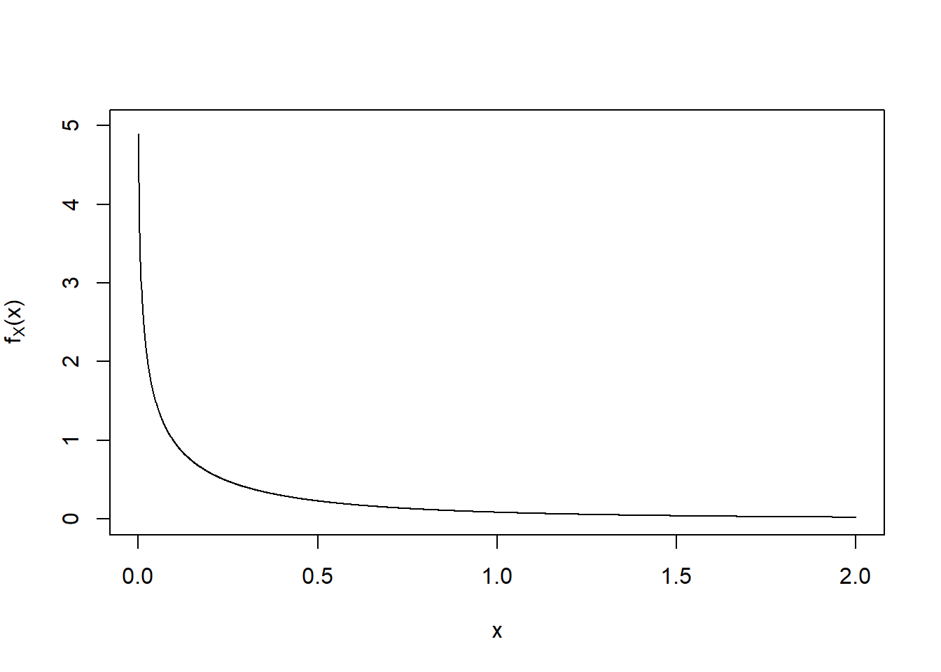

Figure 12.1: Plot of the p.d.f. of $X$.

We consider the link between the conditional expectation of $X$ given $Y$ and the expectation of (the marginal distribution of) $X$.

Tower Property.

Let $X$ and $Y$ be a continuous bivariate distribution with joint p.d.f., $f_{X,Y} (x,y)$. Then $$E [X] = \int_{-\infty}^\infty E[X|Y=y] f_Y (y) \, dy.$$

Note that $$\begin{eqnarray*} E [X] &=& \int_{-\infty}^\infty \int_{-\infty}^{\infty} x f_{X,Y} (x,y) \, dx \, dy \\ &=& \int_{-\infty}^\infty \left[ \int_{-\infty}^{\infty} x f_{X|Y} (x|y) f_Y (y) \, dx \right] \, dy \\ &=& \int_{-\infty}^\infty \left[ \int_{-\infty}^{\infty} x f_{X|Y} (x|y) \, dx \right] f_Y (y) \, dy \\ &=& \int_{-\infty}^\infty E[X|Y=y] f_Y (y) \, dy, \\ \end{eqnarray*}$$

as required.

Therefore in Example 12.2.2, $$\begin{eqnarray*} E [X] &=& \int_{-\infty}^\infty E[X|Y=y] f_Y (y) \, dy, \\ &=& \int_0^\infty y f_Y (y) \, dy \\ &=& E[Y] =1. \end{eqnarray*}$$

This is far simpler than trying to obtain the marginal distribution of $X$ to compute $E[X]$.

12.3 Independent random variables

Recall the definition of independence for random variables given in Section 6.4. If $X$ and $Y$ are independent continuous random variables, then for any $y$ such that $f_Y(y)>0$:
$$f_{X|Y}(x|y) = \frac{f_{X,Y}(x,y)}{f_Y(y)} = \frac{f_X(x)f_Y(y)}{f_Y(y)} = f_X(x), \qquad \mbox{for all }\,x\in\mathbb R.$$

Student Exercise

Attempt the exercise below.

Suppose that the joint probability density function of $X$ and $Y$ is
$$f_{X,Y}(x,y) = \begin{cases} 3y(x+\frac{1}{4}y) & 0 \leq x,y \leq 1 \\ 0 & \text{otherwise.} \end{cases}$$

Find

1. the conditional probability density function of $X$ given $Y=y$, where $y \in (0,1]$,
   
2. $E[X|Y=y],$ for $y \in (0,1]$,
   
3. $P(X>\frac{1}{2} | Y=1)$.
   

Solution to Exercise 12.1.

1. For $y \in [0,1]$,
   $$\begin{eqnarray*} f_Y(y) &=& \int_0^1 3y \left( x + \frac{1}{4}y \right) dx = \left[ 3y \left( \frac{1}{2}x^2 + \frac{1}{4}xy \right) \right]_0^1 \\ &=& 3y \left( \frac{1}{2} + \frac{1}{4}y \right) = \frac{3}{4}y(2+y). \end{eqnarray*}$$ Hence, for $y \in (0,1]$,
   $$\begin{eqnarray*} f_{X|Y}(x|y) &=& \begin{cases} \frac{f_{X,Y}(x,y)}{f_Y(y)}, & 0 \leq x \leq 1, \\ 0 & \text{otherwise,} \end{cases} \\ &=& \begin{cases} \frac{3y(x+\frac{1}{4}y)}{\frac{3}{4}y(2+y)}, & 0 \leq x \leq 1, \\ 0 & \text{otherwise,} \end{cases} \\ &=& \begin{cases} \frac{4x+y}{2+y}, & 0 \leq x \leq 1, \\ 0 & \text{otherwise.} \end{cases} \\ \end{eqnarray*}$$
2. For $y \in (0,1]$,
   $$\begin{eqnarray*} E[X|Y=y] &=& \int_0^1 xf_{X|Y}(x|y) dx \\ &=& \int_0^1 x \frac{4x+y}{2+y} dx = \frac{1}{2+y} \int_0^1 x(4x+y) dx \\ &=& \frac{1}{2+y} \left[ \frac{4}{3}x^3 + \frac{1}{2}x^2y \right]_0^1 = \frac{1}{2+y} \left(\frac{4}{3} + \frac{1}{2}y\right) \\ &=& \frac{8+3y}{6(2+y)}. \end{eqnarray*}$$
3. Fixing $Y=1$, $$\begin{eqnarray*} P\left(\left. X>\frac{1}{2} \right|Y=1\right) &=& \int_{1/2}^1 f_{X|Y}(x|y=1) dx \\ &=& \frac{1}{3} \int_{1/2}^1 (4x+1) dx \\ &=& \frac{1}{3} \left[ 2x^2 + x \right]_{1/2}^1 \\ &=& \frac{1}{3} \left( 2 + 1 - \frac{2}{4} - \frac{1}{2} \right) = \frac{2}{3}. \end{eqnarray*}$$