Code
## run only once (manually)
tbl10 <- readr::read_csv(
    "data/chap10/pew_libraries_2016_cleaned_ch10.csv",
    col_types = "nffffffff"
)

save_data_file("chap10", tbl10, "tbl10.rds")Objectives for chapter 10
SwR Achievements
Harris defines digital divide broader and includes both limited access to information and communication technologies (ICT) and a deficit in the ability to use information gained through access to ICTs1.
People were more likely to fall into this digital divide if they were poor, a racial minority, had limited education, had a disability, or lived in an area with low population density. The digital divide often exacerbated other problems like finding an employment either by not searching relevant offers using the internet or not getting the job because of missing ICT skills.
The question this chapter tries to answer: “Which characteristics are associated with library use?”
Data, codebook, and R packages for learning about descriptive statistics
Data
Two options for accessing the data:
pew_libraries_2016_cleaned_ch10.csv from https://edge.sagepub.com/harris1e.pew_libraries_2016_ch10.csv from https://edge.sagepub.com/harris1e or download from the original Internet data source and clean.I am using the first option because there is nothing new for me to import and clean data files.
Codebook
Two options:
pew_libraries_2016_codebook_ch10.docx codebook file from https://edge.sagepub.com/harris1e.Packages
Example 10.1 : EDA: Get, show and recode data
R Code 10.1 : Import data from .csv file
## run only once (manually)
tbl10 <- readr::read_csv(
"data/chap10/pew_libraries_2016_cleaned_ch10.csv",
col_types = "nffffffff"
)
save_data_file("chap10", tbl10, "tbl10.rds")(For this R code chunk is no output available)
In my first import trial it turned out that all the factor variables are imported as character variables. So I had to add the columns specifications col_types = "nffffffff".
R Code 10.2 : Show raw data for chapter 10
| Name | tbl10 |
| Number of rows | 1601 |
| Number of columns | 9 |
| _______________________ | |
| Column type frequency: | |
| factor | 8 |
| numeric | 1 |
| ________________________ | |
| Group variables | None |
Variable type: factor
| skim_variable | n_missing | complete_rate | ordered | n_unique | top_counts |
|---|---|---|---|---|---|
| sex | 0 | 1.00 | FALSE | 2 | mal: 833, fem: 768 |
| parent | 5 | 1.00 | FALSE | 2 | not: 1205, par: 391 |
| disabled | 8 | 1.00 | FALSE | 2 | no: 1340, yes: 253 |
| uses.lib | 0 | 1.00 | FALSE | 2 | no: 809, yes: 792 |
| ses | 0 | 1.00 | FALSE | 3 | med: 1197, low: 246, hig: 158 |
| raceth | 140 | 0.91 | FALSE | 3 | Non: 1097, His: 194, Non: 170 |
| educ | 0 | 1.00 | FALSE | 3 | HS : 772, Fou: 658, < H: 171 |
| rurality | 14 | 0.99 | FALSE | 3 | rur: 879, sub: 355, urb: 353 |
Variable type: numeric
| skim_variable | n_missing | complete_rate | mean | sd | p0 | p25 | p50 | p75 | p100 | hist |
|---|---|---|---|---|---|---|---|---|---|---|
| age | 30 | 0.98 | 49.31 | 18.85 | 16 | 33 | 51 | 64 | 95 | ▆▅▇▆▁ |
I have used the {skimr} package instead of {tableone}. It wouldn’t be necessary to plot a histogram for age to decide if the mean or median has to be used. The tiny histogram at the right side of the age line already shows that age is not normally distributed. But for the sake of practice I will create the histogram in the next tab.
R Code 10.3 : Show age distribution
my_hist_dnorm(tbl10, tbl10$age)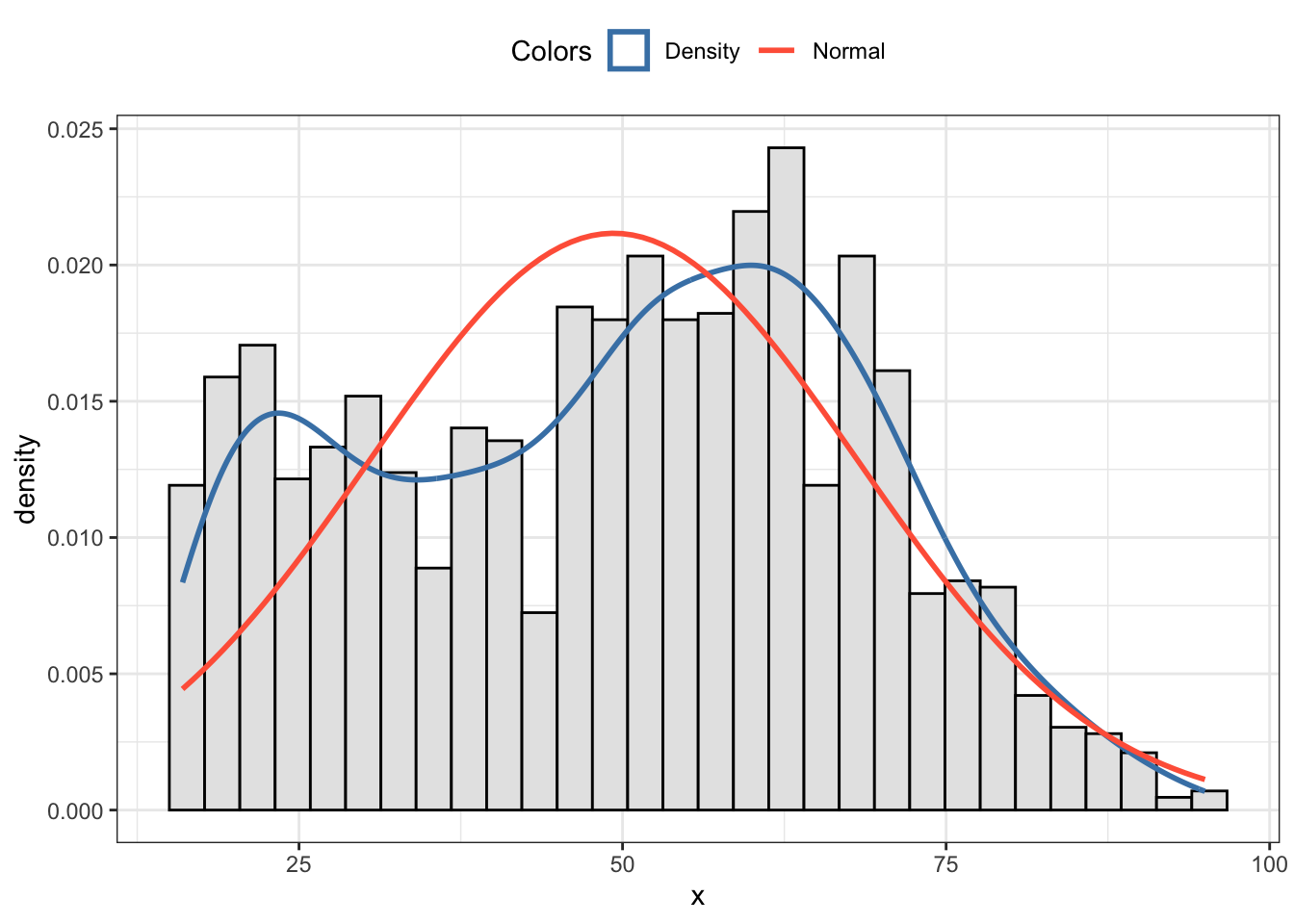
R Code 10.4 : Table of descriptive statistics
tab_desc <- tableone::CreateTableOne(
    data = tbl10,
    strata = 'uses.lib',
    vars = c("age", "sex", "parent", "disabled",
             "ses", "raceth", "educ", "rurality"))

print(tab_desc,
      nonnormal = 'age',
      showAllLevels = TRUE)
#> Stratified by uses.lib
#> level yes
#> n 792
#> age (median [IQR]) 49.00 [31.00, 62.00]
#> sex (%) female 438 (55.3)
#> male 354 (44.7)
#> parent (%) parent 222 (28.2)
#> not parent 566 (71.8)
#> disabled (%) no 679 (86.3)
#> yes 108 (13.7)
#> ses (%) medium 585 (73.9)
#> high 91 (11.5)
#> low 116 (14.6)
#> raceth (%) Non-Hispanic White 540 (75.6)
#> Hispanic 83 (11.6)
#> Non-Hispanic Black 91 (12.7)
#> educ (%) HS to 2-year degree 341 (43.1)
#> Four-year degree or more 382 (48.2)
#> < HS 69 ( 8.7)
#> rurality (%) suburban 196 (24.9)
#> rural 401 (51.0)
#> urban 189 (24.0)
#> Stratified by uses.lib
#> no p test
#> n 809
#> age (median [IQR]) 53.00 [35.00, 65.00] 0.001 nonnorm
#> sex (%) 330 (40.8) <0.001
#> 479 (59.2)
#> parent (%) 169 (20.9) 0.001
#> 639 (79.1)
#> disabled (%) 661 (82.0) 0.024
#> 145 (18.0)
#> ses (%) 612 (75.6) 0.088
#> 67 ( 8.3)
#> 130 (16.1)
#> raceth (%) 557 (74.6) 0.110
#> 111 (14.9)
#> 79 (10.6)
#> educ (%) 431 (53.3) <0.001
#> 276 (34.1)
#> 102 (12.6)
#> rurality (%) 159 (19.9) 0.002
#> 478 (59.7)
#> 164 (20.5)Remark 10.1. : Printing bivariate tests for all variables — a QRP
I am not feeling comfortable to use {tableone} to print descriptive statistics with bivariate test for all variables. Besides the mentioned danger of a questionable research practice (QRP) in looking for statistically significance I would like to inspect the relationships more slowly and to see more details. I think at a minimum one should examine plots of the bivariate correlations.
I have the same skepticism about the advice to “examine the frequencies and percentages in the table to identify some possible categories that may be driving the significant results for the bivariate tests”. I think one should be guided to inspect more in detail in the first instance by theoretical assumptions, an approach that is fairly well demonstrated with Bayesian model design in “Statistical Rethinking” (McElreath 2020).
To facilitate exploratory data analysis one could use packages that combine the analysis of different variables in one go, as my experiments with GGally::ggpairs() in Listing / Output 9.37 or with ggfortify::autoplot() in Listing / Output 9.38 have shown. But this approach gets too overwhelming when there are more than 5-6 variables as I will demonstrate in Listing / Output 10.5 with {GGally).
R Code 10.5 : Bivariate exploratory data analysis for variables of chapter 10
tbl10 |>
    GGally::ggpairs()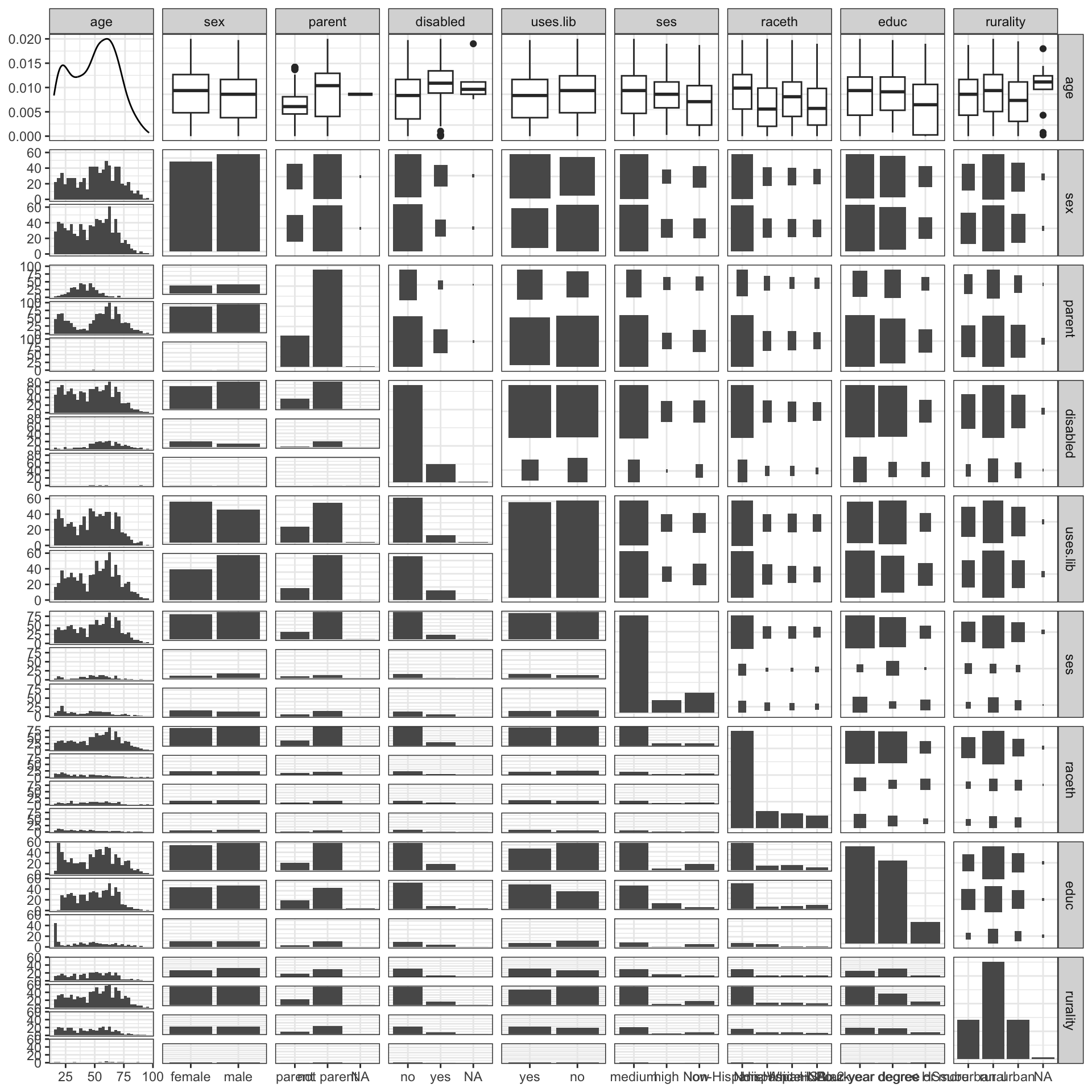
There are too many plots (variables) in this example. I could divide easily the amount of variables into different patches as demonstrated in Columns and Mapping and inspect these results in more details. But in order to get all variations I have to plan the approach systematically which destroys the advantage of automatic plotting.
Binary logistic regression follows a similar format and process as linear regression (Chapter 9), but the outcome or dependent variable is binary. Because the outcome is binary, or categorical consisting of two categories, the model predicts the probability that a person is in one of the two categories. In this chapter we want to predict the library use uses.lib.
Because of the binary outcome the linear regression model would not work since it requires a continuous outcome. However, the linear regression statistical model can be transformed using logit transformations in order to be useful for modeling binary outcomes.
Formula 10.1 : Formula for the statistical form of the logistic model
\[ \begin{align*} p(y) = \frac{1}{1+e^{-(b_{0}+b_{1}x_{1}+b_{2}x_{2})}} \end{align*} \tag{10.1}\]
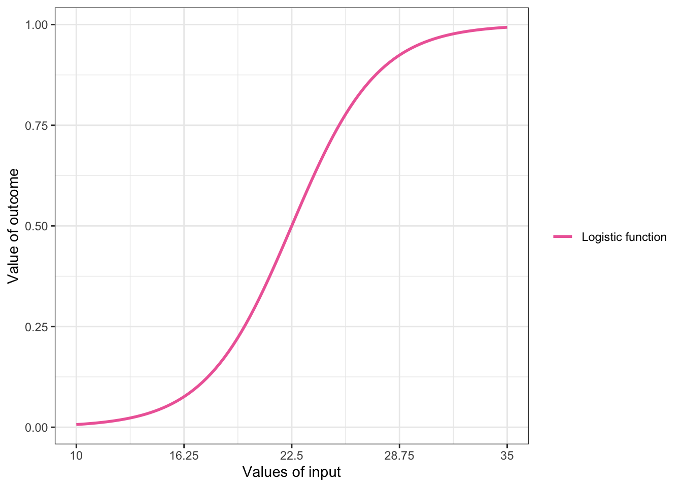
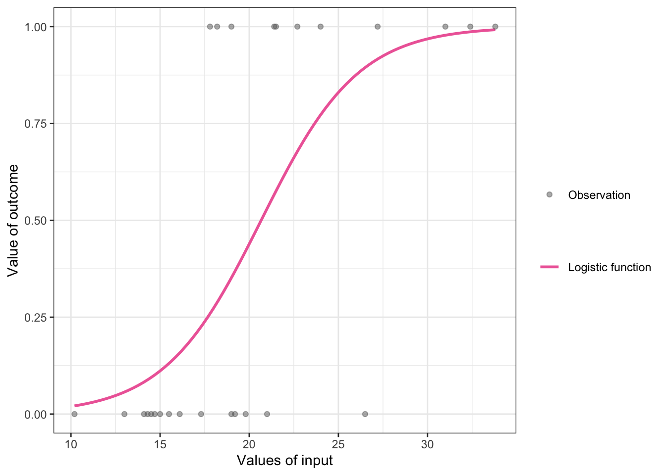
The logistic function has a sigmoid shape that stretches from \(–∞\) to \(∞\) on the x-axis and from \(0\) to \(1\) on the y-axis. The function can take any value along the x-axis and give the corresponding value between \(0\) and \(1\) on the y-axis.
Formula 10.2 : Formula of the logistic function
\[ \begin{align*} \sigma(t) &= \frac{e^t}{1+e^t} =\\ &= \frac{1}{1 + e^{-t}} \end{align*} \tag{10.2}\]
\(t\): value along the \(x\)-axis of the function \(\sigma\): value of \(y\) for a specific value of \(t\), or the probability of \(y\) given \(t\).
In the case of logistic regression, the value of \(t\) will be the right-hand side of the regression model, which looks something like \(β_{0} + β_{1}x\), where \(x\) is an independent variable, \(β_{1}\) is the coefficient (rather than slope) for that variable, and \(β_{0}\) is the constant (rather than \(y\)-intercept).
Substituting this regression model for \(t\) in the logistic function:
\[ \begin{align*} p(y) = \frac{1}{1 + e^{-(β_{0} + β_{1}x)}} \end{align*} \tag{10.3}\]
Example 10.2 : Drawing shape of logistic function empty and with example data points
R Code 10.6 : Shape of the logistic function
ggplot2::ggplot(data = data.frame(x = c(-5, 5)),
         ggplot2::aes(x)) +
    ggplot2::stat_function(fun =
           function(x) base::exp(x)/(1 + base::exp(x)), n = 100,
           linewidth = 1,
           ggplot2::aes(color = "Logistic function")
           ) +
    ggplot2::scale_x_continuous(
        labels = seq.int(10, 35, length.out = 5)
        ) +
    ggplot2::scale_color_manual(
        name = "",
        values = "hotpink2"
    ) +
    ggplot2::labs(
        x = "Values of input",
        y = "Value of outcome"
    )
R Code 10.7 : Example of logistic function with data points
## generate fake data frame
x1 = c(10.2, 13.0, 14.1, 14.3, 14.5, 14.7, 15.0, 15.5,
      16.1, 17.3, 19.0, 19.2, 19.8, 21.0, 26.5)
y1 = rep(0, 15)
x2 = c(17.8, 18.2, 19.0, 21.4, 21.5, 22.7, 24.0, 27.2, 31.0, 32.4, 33.8)
y2 = rep(1, 11)
tbl <-  tibble::tibble(x = c(x1, x2),
                     y = c(y1, y2)) |>
    dplyr::arrange(x)

## draw logistic function with faked data points
ggplot2::ggplot(
        data = tbl,
        ggplot2::aes(x = x, y = y,
                 color = "Logistic function")
    ) +
    ggplot2::stat_smooth(
        data = tbl,
        formula = y ~ x,
        method = "glm",
        se = FALSE,
        method.args = list(family = binomial)
    ) +
    ggplot2::geom_point(
        ggplot2::aes(alpha = "Observation"),
        color = "grey41"
    ) +
    ggplot2::labs(
        x = "Values of input",
        y = "Value of outcome"
    ) +
    ggplot2::scale_color_manual(
        name = "",
        values = "hotpink2"
    ) +
    ggplot2::scale_alpha_manual(
        name = "",
        values = 0.5
    )
R Code 10.8 : Example of logistic function showing probability of outcome for x = 20
## generate fake data frame
x1 = c(10.2, 13.0, 14.1, 14.3, 14.5, 14.7, 15.0, 15.5,
      16.1, 17.3, 19.0, 19.2, 19.8, 21.0, 26.5)
y1 = rep(0, 15)
x2 = c(17.8, 18.2, 19.0, 21.4, 21.5, 22.7, 24.0, 27.2, 31.0, 32.4, 33.8)
y2 = rep(1, 11)
tbl <-  tibble::tibble(x = c(x1, x2),
                     y = c(y1, y2)) |>
    dplyr::arrange(x)

## draw logistic function with faked data points
ggplot2::ggplot(
    data = tbl,
    ggplot2::aes(x = x, y = y,
                 color = "Logistic function")
    ) +
    ggplot2::stat_smooth(
        data = tbl,
        formula = y ~ x,
        method = "glm",
        se = FALSE,
        method.args = list(family = binomial),
        ggplot2::aes(linetype = "predictor = 20 and\noutcome = .44 example")
    ) +
    ggplot2::geom_point(
        ggplot2::aes(alpha = "Observation"),
        color = "grey41"
        ) +
    ggplot2::geom_segment(
        x = 20, xend = 20,
        y = 0, yend = .44,
        color = "#1f6fca",
        linetype = "dashed"
    ) +
    ggplot2::geom_segment(
        x = 10, xend = 20,
        y = .44, yend = .44,
        color = "#1f6fca",
        linetype = "dashed"
    ) +
    ggplot2::labs(
        x = "Values of input",
        y = "Value of outcome"
    ) +
    ggplot2::scale_color_manual(
        name = "",
        values = "hotpink2"
    ) +
    ggplot2::scale_alpha_manual(
        name = "",
        values = 0.5
    ) +
    ggplot2::scale_linetype_manual(
        name = "",
        values = c("dashed", "dashed")
    ) +
    ggplot2::annotate("text", x = 10, y = .48, label = "0.44", color = "#1f6fca" ) +
    ggplot2::annotate("text", x = 20.5, y = -.02, label = "20", color = "#1f6fca" )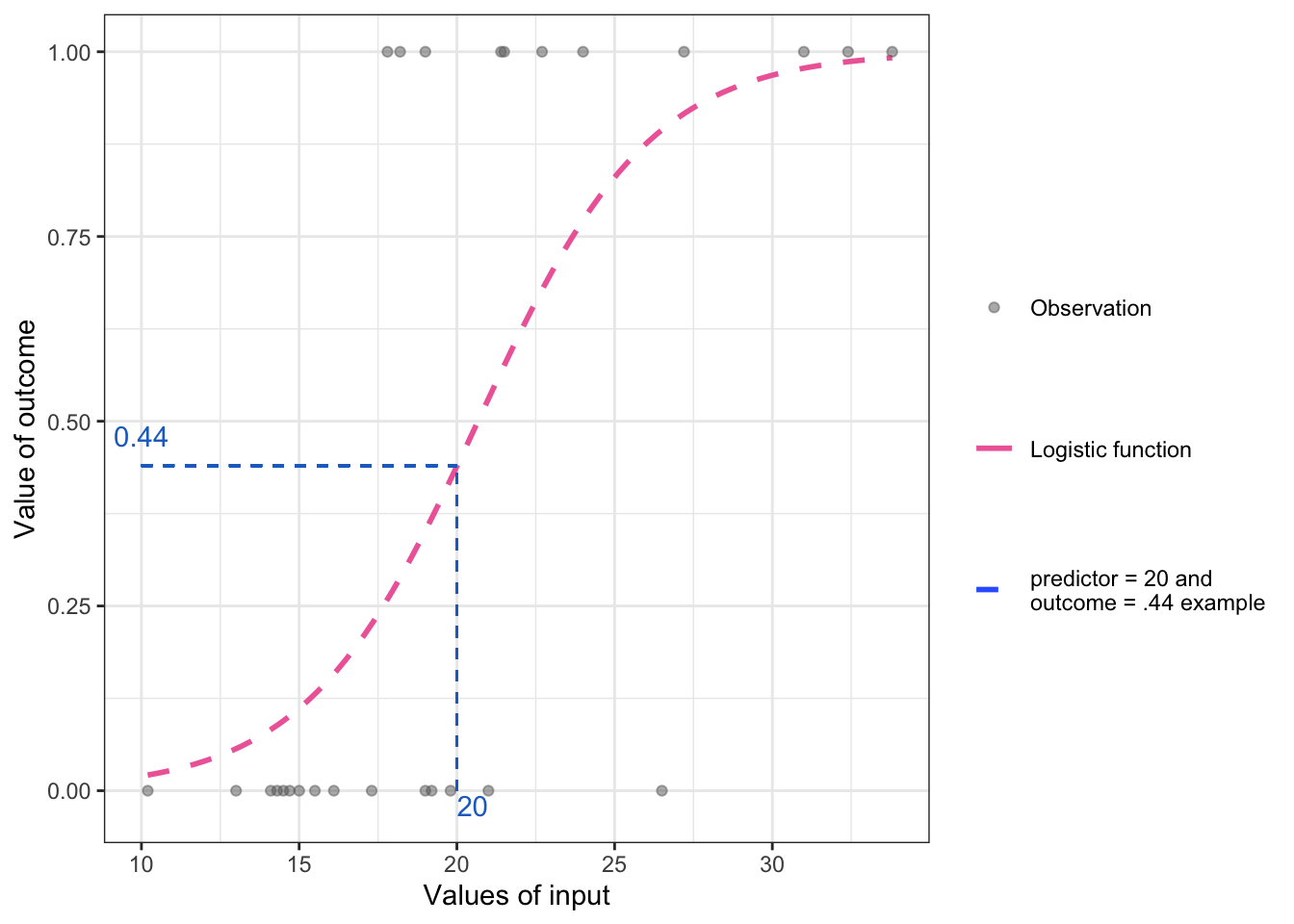
Let’s assume that the above graphic is a model for predicting library use from age. Then we can interpret it as a 44% probability of library use for a 20-year-old. Since 44% is lower than a 50% probability of the value of \(y\), the model is predicting that the 20-year-old does not have the outcome. So, if the outcome is library use, the logistic model would predict this 20-year-old was not a library user.
Formula 10.3 : Formula of odds related to probability
\[ \begin{align*} odds = \frac{probability}{1-probability} \end{align*} \tag{10.4}\]
Substituting the logistic model from Equation 10.1:
\[ \begin{align*} odds &= \frac{\frac{1}{1+e^{-(\beta_{0}+\beta_{1}x)}}}{1- \frac{1}{1+e^{-(\beta_{0}+\beta_{1}x)}}} = e^{\beta_{0} + \beta_{1}x} \end{align*} \tag{10.5}\]
To be equivalent to the interpretation of the coefficients in linear regression, however, there is one more step. That is, what is the increase or decrease in the odds of the outcome with a one-unit increase in \(x\)?
\[ \begin{align*} OR = \frac{e^{b_0+b_{1}(x+1)}}{e^{b_0+b_{1}x}} \end{align*} \tag{10.6}\]
Equation 10.6 shows that for every one-unit increase in the independent variable \(x\), the odds of the outcome increase or decrease by \(e^{b_1}\). Taking \(e\) to the power of \(b_1\) is referred to as exponentiating \(b_1.\) After a model is estimated, the analyst will usually exponentiate the b value(s) in order to report odds ratios describing the relationships between each predictor and the outcome.
Write the null and alternate hypotheses:
Compute the test statistic.
The generalized linear model (GLM) or stats::glm() function can be used to estimate a binary logistic regression model. The model is generalized because it starts with the basic linear model and generalizes to other situations.
The stats::glm() function will treat the first category as the reference group (the group without the outcome) and the second category as the group with the outcome. To see the order of uses.lib, use base::levels() to show the levels in order and use stats:relevel() to re-order levels.
Example 10.3 : Numbered Example Title
R Code 10.9 : Reverse the order of uses.lib
glue::glue("Order of uses.lib levels originally")
base::levels(tbl10$uses.lib)

tbl10.1 <- tbl10 |>
    dplyr::mutate(uses.lib =
        forcats::fct_rev(uses.lib)
    )

save_data_file("chap10", tbl10.1, "tbl10.1.rds")


glue::glue("")
glue::glue("---------------------------------------")
glue::glue("Order of uses.lib levels reversed")
base::levels(tbl10.1$uses.lib)
#> Order of uses.lib levels originally
#> [1] "yes" "no"
#>
#> ---------------------------------------
#> Order of uses.lib levels reversed
#> [1] "no" "yes"uses.lib
In contrast to the book the order of my levels for the uses.lib data is reversed. It makes more sense to ask about if one uses the library, e.g., “yes” has to be the second category. To get the same order as in the book, I had to reverse the order. Instead of using stats:relevel() I reversed the order with forcats::fct_rev().
R Code 10.10 : Estimate library use model and print results
#>
#> Call:
#> glm(formula = uses.lib ~ age, family = binomial(link = "logit"),
#>     data = tbl10.1)
#>
#> Coefficients:
#>              Estimate Std. Error z value Pr(>|z|)
#> (Intercept)  0.403785   0.142194   2.840  0.00452 **
#> age         -0.008838   0.002697  -3.277  0.00105 **
#> ---
#> Signif. codes:  0 '***' 0.001 '**' 0.01 '*' 0.05 '.' 0.1 ' ' 1
#>
#> (Dispersion parameter for binomial family taken to be 1)
#>
#>     Null deviance: 2177.5  on 1570  degrees of freedom
#> Residual deviance: 2166.7  on 1569  degrees of freedom
#>   (30 observations deleted due to missingness)
#> AIC: 2170.7
#>
#> Number of Fisher Scoring iterations: 3
Listing / Output 10.10 uses stats::family = binomial(link = "logit")to specify the outcome variable. The “family” argument provides a description of the error distribution and link function to be used in the model. This is a convenient way to specify the details of the models and to distinguish between different types of generalized linear models that are appropriate for different kinds of outcome variables. In addition to the glm() help page you get additional information if you type ?family into the console.
stats::-prefix in front of glm() in later R code
Because of an error in the coding of the DescTools::PseudoR2() function I had to delete my stats::-prefix in front of the glm() function in Listing / Output 10.10. (See Warning 10.2)
R Code 10.11 : Get model fit, model significance, and odds ratios
odds.n.ends::odds.n.ends(glm10.1)#> Waiting for profiling to be done...#> $`Logistic regression model significance`
#> Chi-squared d.f. p
#> 10.815 1.000 0.001
#>
#> $`Contingency tables (model fit): frequency predicted`
#> Number observed
#> Number predicted 1 0 Sum
#> 1 338 298 636
#> 0 435 500 935
#> Sum 773 798 1571
#>
#> $`Count R-squared (model fit): percent correctly predicted`
#> [1] 53.34182
#>
#> $`Model sensitivity`
#> [1] 0.4372574
#>
#> $`Model specificity`
#> [1] 0.6265664
#>
#> $`Predictor odds ratios and 95% CI`
#> OR 2.5 % 97.5 %
#> (Intercept) 1.497482 1.1339164 1.9804811
#> age 0.991201 0.9859589 0.9964415Review and interpret the test statistics: Calculate the probability that your test statistic is at least as big as it is if there is no relationship (i.e., the null is true).
Example 10.4 : Chi-squared distribution with df = 1
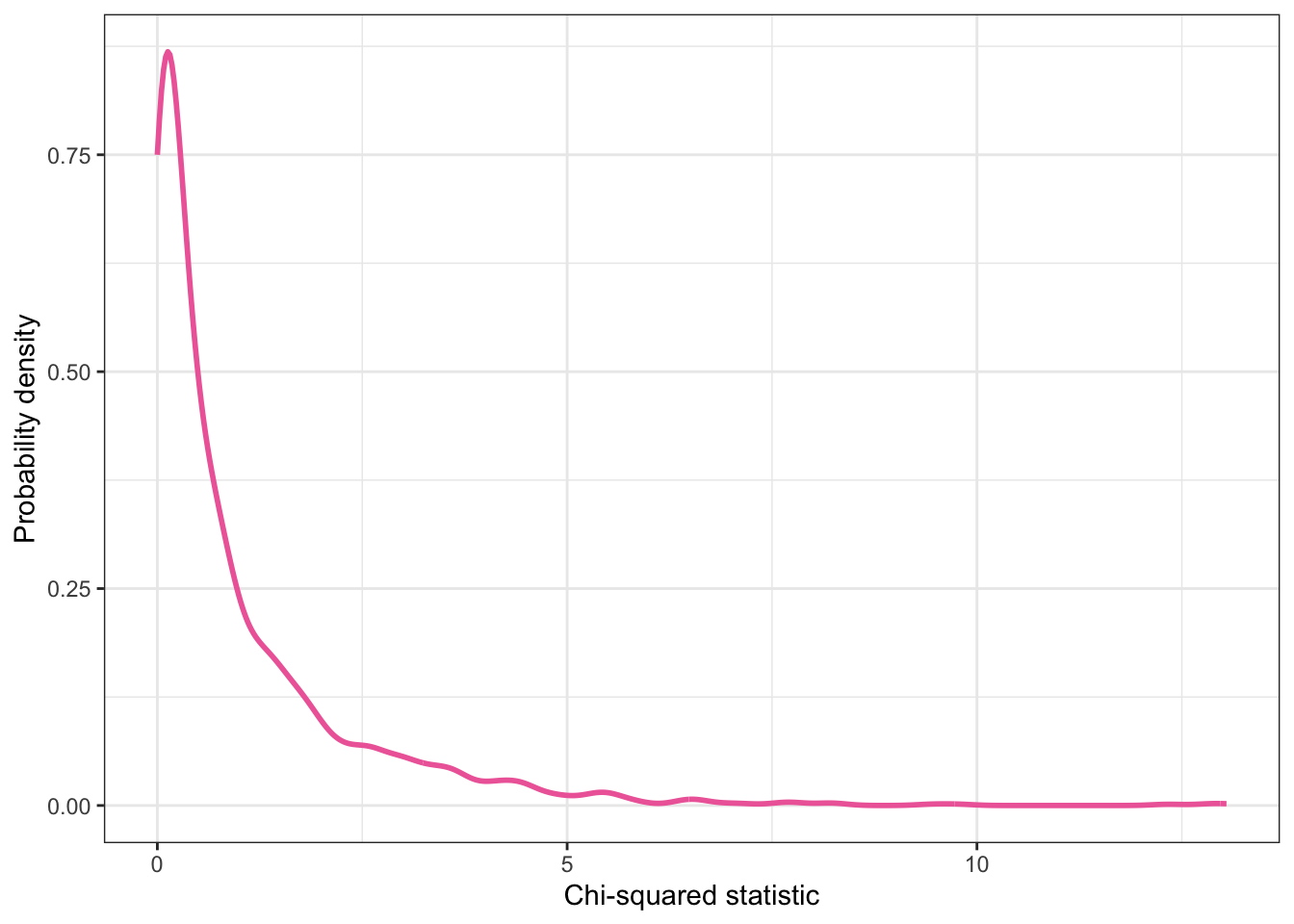
R Code 10.12 : Theoretical chi-squared distribution with df = 1
ggplot2::ggplot() +
    ggplot2::xlim(0, 12) +
    ggplot2::stat_function(
        fun = dchisq,
        args = list(df = 1),
        linewidth = 1,
        color = "hotpink2"
    ) +
    ggplot2::labs(
        x = "Chi-squared statistic",
        y = "Probability density"
    )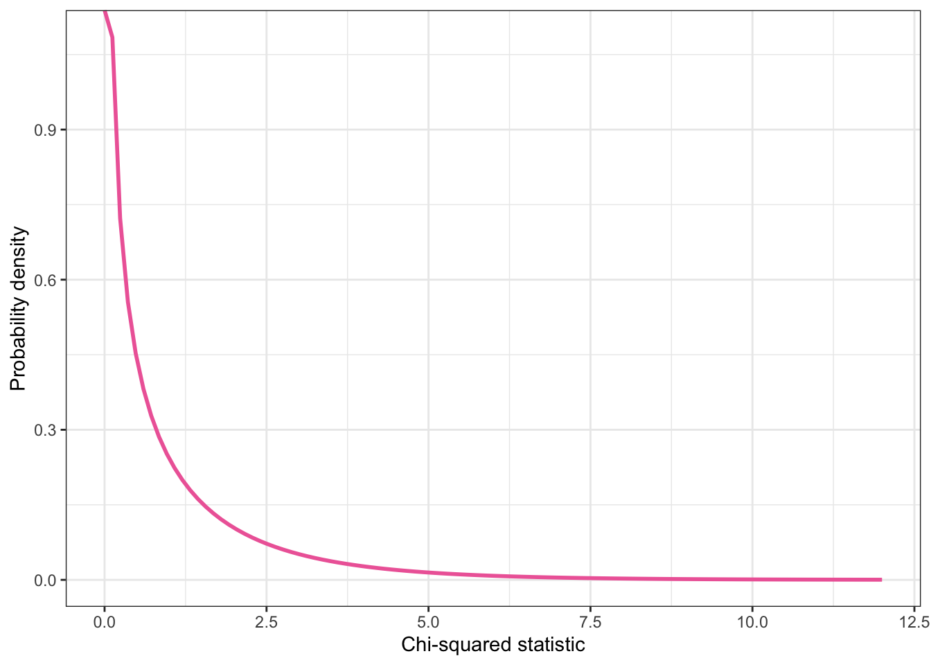
Graphing the probability of the chi-squared distribution with 1 degree of freedom to show that the probability that the chi-squared would be 10.815 or higher — if the null hypothesis were true — is the very small area under the curve from 10.815 to the right.
To get a better look at the position \(x = 10.815\) let’s zoom into the critical region. See Listing / Output 10.13.
R Code 10.13 : Theoretical chi-squared distribution with df = 1, zoomed into the critical region of p = 10.815
## Define start of shade
x_shade = 10.815
df = 1
y_shade = stats::dchisq(x_shade, df)


## Define sequence of x-values
tib <- tibble::tibble(x = seq(9, 20, length.out = 300)) |>
    # Compute density values
    dplyr::mutate(
        y = stats::dchisq(x, df)
    )

## Subset data for shaded area
shaded_area <- tib |>
    dplyr::filter(x >= x_shade) |>
    ## Necessary as starting point for y = 0!
    tibble::add_row(x = x_shade, y = 0, .before = 1)


tib |>
    ## Plot the Chi-square distribution: df = 1
    ggplot2::ggplot(ggplot2::aes(x = x, y = y)) +
    ggplot2::geom_line(
        linewidth = 1,
        color = "hotpink2"
    ) +

    ## Draw segment
    ggplot2::geom_segment(
        x = x_shade,
        y = 0,
        xend = x_shade,
        yend = y_shade
    ) +

    ## Shade curve
    ggplot2::geom_polygon(
        data = shaded_area,
        fill = "lightblue",
        ggplot2::aes(x = x, y = y)
        ) +
    ggplot2::labs(
        x = "Chi-squared statistic",
        y = "Probability density"
    ) +
    ggplot2::annotate(
        geom = "text",
        x = 11.5,
        y = .00058,
        label = base::round(stats::dchisq(x_shade, df), 6)
    )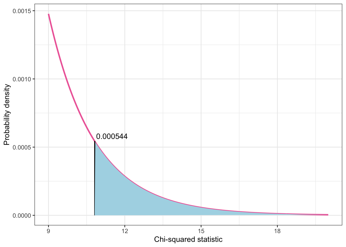
Here we see that at the chi-square statistic of 10.815 the p-value is with .0005 very tiny and about 100 times much smaller as the level of statistical significance of .05.
When I developed above plots I wondered why in the book the graph is a rough line and the sample size (without NA’s) of \(n = 1501\) was mentioned. I learned that my curve was the theoretical curve whereas I need the randomized values to get a more rough simulation that is nearer the factual data.
R Code 10.14 : Randomized chi-squared distribution with df = 1, n = 1571
This is a randomized chi-squared distribution. I could not shade values \(p > 10.815\) because there were only three rows with values greater than that.
TODO: I wonder if I could provide an empirical chi-squared distribution with the actual data.
Resource 10.1 : Video about the chi-squared distribution
I found a lengthy video tutorial (19:31) using RStudio featuring chi-squared distribution. You will see, pdf, cdf, quantile, plotting, examples, independence, goodness of fit and explanations. There is also a accompanying web page with text and the code.
Conclude and write report.
Both, base::summary() and odds.n.ends::odds.n.ends() included values and significance statistics for the age predictor. The odds.n.ends() output included odds ratios, which are easier to interpret. The outcome is transformed by the logistic function, therefore the coefficients from summary() are not easy to interpret directly.
Looking at Listing / Output 10.11 we see that agehas a odds ratio of .99. This could be interpreted as, “The odds of library use decrease by 1% for every 1-year increase in age.” The 1% comes from subtracting the odds ratio of .99 from 1 and multiplying by 100 to convert it to a percent. This is a stategy to make interpreting odds below 1 easier. Otherwise we would have to say: “The odds of library use are .99 times as high with every 1-year increase in age.”
When the confidence interval includes 1, the odds of the outcome are not statistically significantly different with a change in the independent variable.
The odds ratio for the age variable is less than 1, and the confidence interval does not include 1. Thus, the interpretation of this odds ratio would be as follows:
Write the null and alternate hypotheses:
Compute the test statistic.
The base::summary() function following a stats::glm() function includes a z-statistic comparing the coefficient estimate to zero. The z-score is a measure how many standard deviations away a value is from a mean. But for logistic regression, the coefficient divided by the standard error — not by the standard deviation — follows a z-distribution. This z-statistic is the test statistic for the Wald test, which has the same purpose (but follows a different distribution) as the Wald test from Section 9.7.
In the case of the age variable, dividing the estimate of \(-0.008838\) by its standard error of \(0.002697\) gives a z-statistic of \(-3.276974\), which is well beyond the boundary of \(–1.96\) for statistical significance when \(\alpha\) is set at \(.05\).
The z-distribution is a normal distribution with a mean of 0 and a standard deviation of 1.
R Code 10.15 : z-distribution for sample size of 1571
nhstplot::plotztest(
    z = -3.28,
    tails = "one",
    xmax = 5
    )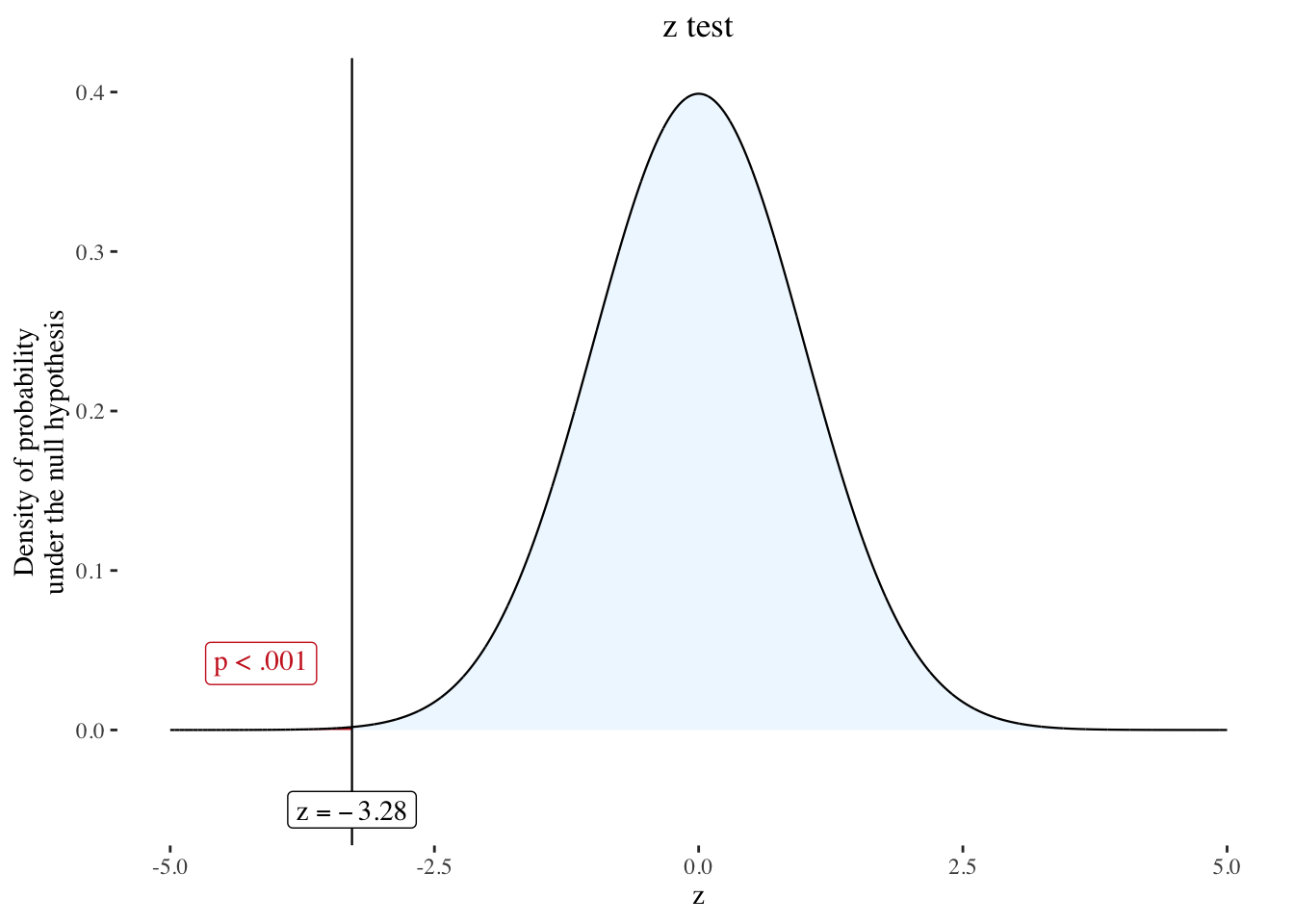
Review and interpret the test statistics: Calculate the probability that your test statistic is at least as big as it is if there is no relationship (i.e., the null is true).
The area under the curve to the left of the test statistic in Listing / Output 10.15 is very small. Given this area is very small, the p-value of .00105 in the output Listing / Output 10.10 from base::summary(glm10.1) makes sense. There is a .105% probability that this sample came from a population where there was no relationship between age and library use. Thus, there is a statistically significant relationship between age and library use (z = –3.28; p = .001).
Conclude and write report.
The odds ratio for age is .99 with a 95% CI of .986–.996. The confidence interval shows the range where the odds ratio likely is in the population. Because the confidence interval does not include 1, this indicates that the odds ratio is statistically significantly different from 1. The interpretation would be as follows:
For linear regression, the \(R^2\) statistic measured how well the model fit the observed data by measuring how much of the variability in the outcome was explained by the model. The concept of variance is appropriate for continuous but not categorical variables. There are several measures for categorical model fit, including the percent correctly predicted, sometimes called count \(R^2\) and the adjusted count \(R^2\), which adjusts the count \(R^2\) for the number of people in the largest of the two categories of the outcome.
The percent correctly predicted by the model is computed using the predicted probabilities, or fitted values, for each of the observations and comparing these probabilities to the true value of the outcome.
Formula 10.4 : Percent correctly predicted or count \(R^2\)
\[ \begin{align*} R^2_{count} = \frac{n_{correct}}{n_{total}} \end{align*} \tag{10.7}\]
For example, if a person in the data set were predicted to have a chance of more than 50% of library use, this would be transformed into a “yes” or “1” value of the outcome and then compared to the person’s actual library use. If the predicted value and the true value matched, this would be considered a correct prediction. The same vice-versa for predicted values less than 50%. The total number of people the model gets correct out of the total number of people in the data analyzed is the percent correctly predicted or count \(R^2\).
The Listing / Output 10.11 includes a table showing how many observations were correctly predicted in each category of the outcome.
Formula 10.5 : Calculate the percent correctly predicted with the glm10.1 data
\[ \begin{align*} R^2_{count} = \frac{338 + 500}{1571} = \frac{838}{1571} = 0.5334 \end{align*} \tag{10.8}\]
An alternative measure of percent correctly predicted is the adjusted count R^2 measure. It adjusts the count \(R^2\) for the number of people in the largest of the two categories of the outcome.
Formula 10.6 : Adjusted count \(R^2\)
\[ \begin{align*} R^2_{count.adj} = \frac{n_{correct}- n_{most.common.outcome}}{n_{total}- n_{most.common.outcome}} \end{align*} \tag{10.9}\]
The argument behind this adjustment is that a null model, or a model with no predictors, could get a good percent correctly predicted just by predicting everyone was in the outcome category that had the bigger percentage of people in it.
For the library use data, the most common category is library nonuse (or 0), with 798 of the 1571 participants with complete data for the model. Without knowing anything about library use, you could predict everyone in the data set was a nonuser and be right \(\frac{788}{1571}\) or 50.8% of the time. Using the age predictor, the model is right \(\frac{338+500}{1571}\) or 53% of the time. While this is not a huge increase, it did classify 40 additional people correctly compared to using the percentages in the outcome categories with no other information.
The model using age to predict library use was correct 53% of the time (Count \(R^2\) = .53). The adjusted count \(R^2\) would be \(\frac{338+500-798}{1571-798}\) or .05.
Pseudo-\(R^2\) is another measure that are reported relatively frequently. This measure generally tries to quantify the reduction in lack of fit between a null and full model. You can compute Pseudo-\(R^2\)
: Packages with function for computing pseudo-\(R^2\)
PseudoR2() from the {DescTools} package (see: Section A.15),lrm()(instead of the stats::glm()!) from the {rms} package (see: Section A.73)pR2()from the {pscl} package (see: Section A.66), andMany of these packages have also function for percent correctly predicted and the adjusted count \(R^2\) measure.
Resource 10.2 : Interpreting the different Pseudo-\(R^2\)
There are many different pseudo-\(R^2\) measures with different theoretical approaches. Therefore also the interpretation of these measures differ.
The best resource I found to explain these differences: FAQ: What are pseudo R-squareds? (UCLA 2011).
But even in this resource not all different pseudo-\(R^2\) measures are explained. Anyway it is an complex issues where I have to spend more time to study the details.
Even in Resource 10.2 not all different pseudo-\(R^2\) measures are explained. It is an complex issues where I have to spend more time to study the details.
Example 10.5 : Computing Pseudo \(R^2\) with different packages
R Code 10.16 : Computing Pseudo-\(R^2\)
DescTools::PseudoR2(
    x = glm10.1,
    which = "all")
#> McFadden McFaddenAdj CoxSnell Nagelkerke AldrichNelson
#> 4.966964e-03 3.129970e-03 6.860773e-03 9.148470e-03 6.837345e-03
#> VeallZimmermann Efron McKelveyZavoina Tjur AIC
#> 1.177035e-02 6.845171e-03 8.360693e-03 6.856907e-03 2.170655e+03
#> BIC logLik logLik0 G2
#> 2.181374e+03 -1.083328e+03 -1.088735e+03 1.081542e+01DescTools::PseudoR2() throws an error message
From DescTools::PseudoR2() I got always the error that the function stats::glm()was not known. After two hours of trials I learned that the function was not programmed for the case that you provide the package name in front of the glm()function. After I deleted this prefix in Listing / Output 10.10 the DescTools::PseudoR2() function worked. (See also Warning 10.1)
R Code 10.17 : Computing Pseudo-\(R^2\) with {performance}
performance::r2(glm10.1)#> # R2 for Logistic Regression
#> Tjur's R2: 0.007performance::r2_tjur(glm10.1)#> Tjur's R2
#> 0.006856907performance::r2_mcfadden(glm10.1)#> # R2 for Generalized Linear Regression
#> R2: 0.024
#> adj. R2: 0.023performance::r2_coxsnell(glm10.1)#> Cox & Snell's R2
#> 0.006860773performance::r2_nagelkerke(glm10.1)#> Nagelkerke's R2
#> 0.00914847performance::r2_efron(glm10.1)#> [1] 0.006845171performance::r2_mckelvey(glm10.1)#> McKelvey's R2
#> 0.008360693R Code 10.18 : Computing Pseudo-\(R^2\) with {rms}
rms::lrm(
    formula = uses.lib ~ age,
    data = tbl10.1
)
#> Frequencies of Missing Values Due to Each Variable
#> uses.lib age
#> 0 30
#>
#> Logistic Regression Model
#>
#> rms::lrm(formula = uses.lib ~ age, data = tbl10.1)
#>
#>
#> Model Likelihood Discrimination Rank Discrim.
#> Ratio Test Indexes Indexes
#> Obs 1571 LR chi2 10.82 R2 0.009 C 0.548
#> no 798 d.f. 1 R2(1,1571)0.006 Dxy 0.096
#> yes 773 Pr(> chi2) 0.0010 R2(1,1178)0.008 gamma 0.097
#> max |deriv| 3e-12 Brier 0.248 tau-a 0.048
#>
#> Coef S.E. Wald Z Pr(>|Z|)
#> Intercept 0.4038 0.1422 2.84 0.0045
#> age -0.0088 0.0027 -3.28 0.0010R Code 10.19 : Computing Pseudo-\(R^2\) with {pscl}
pscl::pR2(glm10.1)#> fitting null model for pseudo-r2#> llh llhNull G2 McFadden r2ML
#> -1.083328e+03 -1.088735e+03 1.081542e+01 4.966964e-03 6.860773e-03
#> r2CU
#> 9.148470e-03R Code 10.20 : Computing Pseudo-\(R^2\) with {pubh}
pubh::pseudo_r2(glm10.1)#> Index Estimate
#> 1 Nagelkerke 0.009
#> 2 Hosmer and Lemeshow 0.005
#> 3 Cox and Snell 0.007Sometimes it is useful to know whether the model is better at predicting people with the outcome or people without the outcome. The measures used for these two concepts are sensitivity and specificity.
Sensitivity determines the percentage of the 1s or “yes” values the model got correct, while specificity computes the percentage of 0s or “no” values the model got correct.
In Listing / Output 10.11, the sensitivity is 43.7% while the specificity is 62.7%. The model was better at predicting the “no” values than the “yes” values. These percentages could also be computed from the frequency table in the output: The model predicted 500 of the 798 people in the 0 category correctly (62.7%) and 338 of the 773 in the 1 category correctly (43.7%).
Example 10.6 : Compute full logistic regression model
R Code 10.21 : Compute full logistic regression model, first try (glm10.2)
# estimate the full library use model and print results
glm10.2 <- glm(
    formula = uses.lib ~ age + sex + educ + parent +
         disabled + rurality + raceth + ses,
         data = tbl10.1,
         na.action = na.exclude,
         family = binomial("logit"))

odds.n.ends::odds.n.ends(glm10.2)
#> Waiting for profiling to be done...#> $`Logistic regression model significance`
#> Chi-squared d.f. p
#> 94.736 12 <.001
#>
#> $`Contingency tables (model fit): frequency predicted`
#> Number observed
#> Number predicted 1 0 Sum
#> 1 378 249 627
#> 0 318 482 800
#> Sum 696 731 1427
#>
#> $`Count R-squared (model fit): percent correctly predicted`
#> [1] 60.26629
#>
#> $`Model sensitivity`
#> [1] 0.5431034
#>
#> $`Model specificity`
#> [1] 0.6593707
#>
#> $`Predictor odds ratios and 95% CI`
#> OR 2.5 % 97.5 %
#> (Intercept) 2.5374457 1.5934592 4.0590559
#> age 0.9899123 0.9835415 0.9962814
#> sexmale 0.4891734 0.3921079 0.6091430
#> educFour-year degree or more 1.6592450 1.3037357 2.1140981
#> educ< HS 0.8714204 0.5900475 1.2806573
#> parentnot parent 0.7903350 0.6060517 1.0297999
#> disabledyes 0.8003756 0.5836481 1.0949054
#> ruralityrural 0.8403500 0.6367719 1.1086567
#> ruralityurban 1.0336350 0.7397448 1.4447031
#> racethHispanic 0.7602893 0.5367016 1.0738082
#> racethNon-Hispanic Black 1.1814334 0.8363155 1.6717295
#> seshigh 1.1804392 0.8037360 1.7398860
#> seslow 1.1005903 0.7957933 1.5220253glm2)
My values are quite different than the outcome in the book. The reason is that I have the levels ordered differently. I will order my levels so that I get the same result as in the book.
R Code 10.22 : Order level to match the result from the book
tbl10.3 <- tbl10.1 |>
    dplyr::mutate(educ =
        forcats::fct_relevel(educ, "< HS", "Four-year degree or more",
                             "HS to 2-year degree")
    ) |>
    dplyr::mutate(parent =
        forcats::fct_rev(parent)
    ) |>
    dplyr::mutate(rurality =
        forcats::fct_relevel(rurality, "rural", "suburban", "urban")
    ) |>
    dplyr::mutate(raceth =
        forcats::fct_relevel(raceth, "Hispanic",
                 "Non-Hispanic Black", "Non-Hispanic White")
    ) |>
    dplyr::mutate(ses =
        forcats::fct_relevel(ses, "high",
                 "low", "medium")
    )

save_data_file("chap10", tbl10.3, "tbl10.3.rds")ses not ordered to their intrinsically ordering?
I have ordered the levels to match the book outcome. But I do not understand why some of the levels (educ, rurality or ses) are not ordered from high to low or vice versa. The highest or lowest level is in the order of the book always in the middle.
R Code 10.23 : Compute full logistic regression model, final version (glm10.3)
# estimate the full library use model
# matching the level order from the book
# and print results with odds.n.ends()

glm10.3 <- glm(
    formula = uses.lib ~ age + sex + educ + parent +
         disabled + rurality + raceth + ses,
         data = tbl10.3,
         na.action = na.exclude,
         family = binomial("logit"))

save_data_file("chap10", glm10.3, "glm10.3.rds")

odds.n.ends::odds.n.ends(glm10.3)
#> Waiting for profiling to be done...#> $`Logistic regression model significance`
#> Chi-squared d.f. p
#> 94.736 12 <.001
#>
#> $`Contingency tables (model fit): frequency predicted`
#> Number observed
#> Number predicted 1 0 Sum
#> 1 378 249 627
#> 0 318 482 800
#> Sum 696 731 1427
#>
#> $`Count R-squared (model fit): percent correctly predicted`
#> [1] 60.26629
#>
#> $`Model sensitivity`
#> [1] 0.5431034
#>
#> $`Model specificity`
#> [1] 0.6593707
#>
#> $`Predictor odds ratios and 95% CI`
#> OR 2.5 % 97.5 %
#> (Intercept) 1.3180091 0.6778733 2.5644803
#> age 0.9899123 0.9835415 0.9962814
#> sexmale 0.4891734 0.3921079 0.6091430
#> educFour-year degree or more 1.9040694 1.2584331 2.8953329
#> educHS to 2-year degree 1.1475517 0.7808490 1.6947789
#> parentparent 1.2652862 0.9710624 1.6500243
#> disabledyes 0.8003756 0.5836481 1.0949054
#> ruralitysuburban 1.1899804 0.9019925 1.5704210
#> ruralityurban 1.2300055 0.9281956 1.6307183
#> racethNon-Hispanic Black 1.5539262 1.0018330 2.4167032
#> racethNon-Hispanic White 1.3152888 0.9312650 1.8632329
#> seslow 0.9323567 0.5720558 1.5162449
#> sesmedium 0.8471423 0.5747503 1.2441896glm10.3)
na.action = na.omit instead of na.action = na.exlcude
To find influential values I have tried several different packages. Using {glmtoolbox} I received an error message when I used na.action = na.exlcude. In the help file to the influence() function I learned:
Cases omitted in the fit are omitted unless a
na.actionmethod was used (such asna.exclude) which restores them. … If a model has been fitted withna.action = na.exclude(seena.exclude), cases excluded in the fit are considered here.
This is a weird behavior because I thought that na.exclude will exclude and not restore the NA-values. But if I tried to change therefore to na.action = na.omit I got an error message in Listing / Output 10.27: “res_std must be size 1601 or 1, not 1427.”
Finally I decided to stick with na.action = na.exclude (or to delete this line completely with the same result) and not to use the {glmtoolbox} package.
Write the null and alternate hypotheses:
Compute the test statistic.
The chi-squared test statistic of 94.74 was computed by the odds.n.ends() function.
R Code 10.24 : Visualizing a chi-squared distribution with n = 1427, df = 12 and test statistic of 94.74
nhstplot::plotchisqtest(
    chisq = 94.74,
    df = 12
)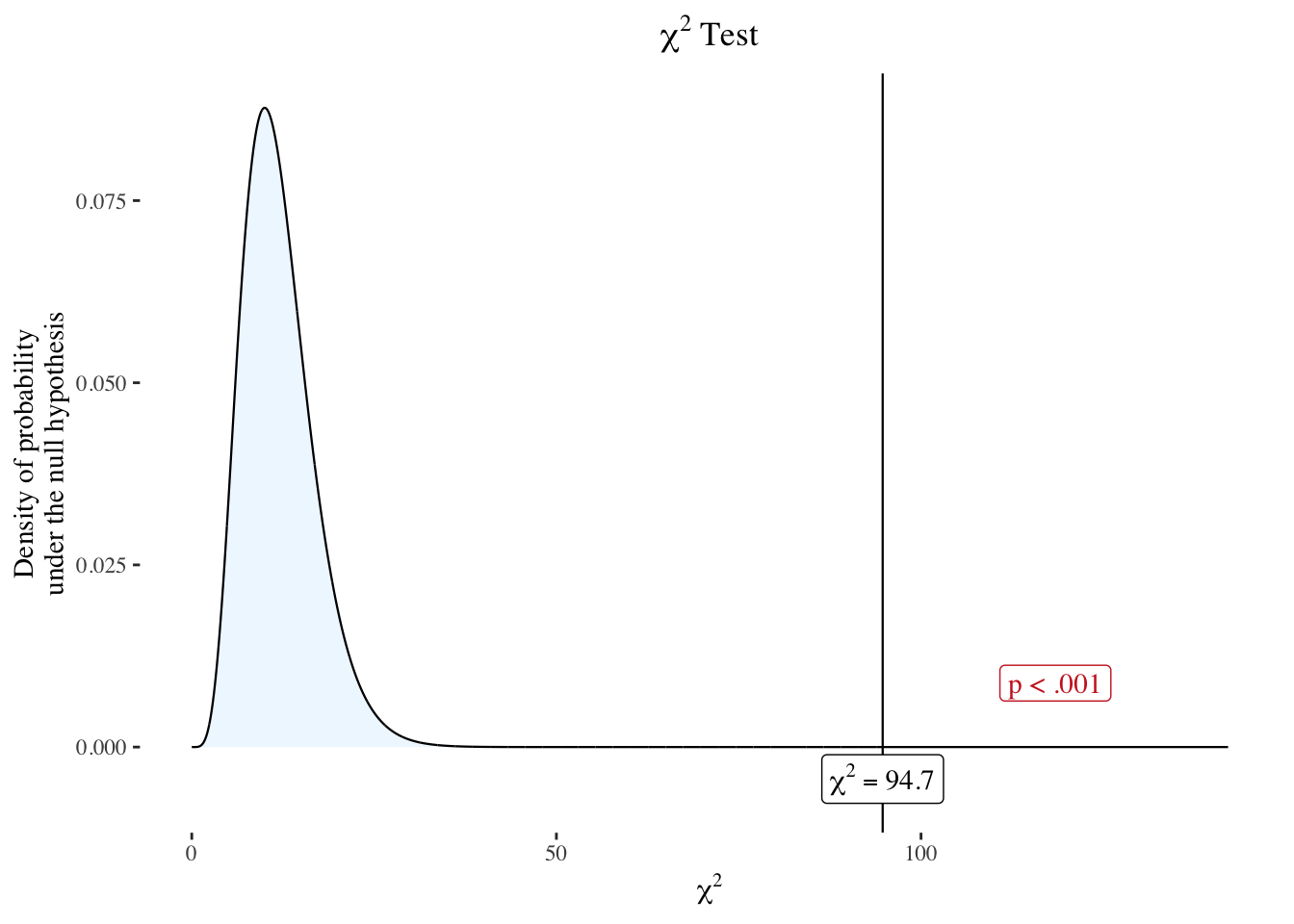
Review and interpret the test statistics: Calculate the probability that your test statistic is at least as big as it is if there is no relationship (i.e., the null is true).
The probability that the chi-squared would be 94.74 if the full model were no better than the null model is shown as the area under the curve to the right starting at 94.74. This corresponds with a very small p-value < .001.
Conclude and write report.
Listing / Output 10.21 includes the odds ratio which are easier to interpret as the significance statistics for the predictors. When the confidence interval includes 1, the odds ratio could be 1 and this indicates it is not statistically significantly different from 1. If the odds ratio is greater than 1 and the confidence interval does not include 1, the odds ratio suggests a statistically significant increase in the odds of the outcome.
Factor variables with two categories were interpreted with respect to the reference group, or the group not shown in the output. Since the factor variables can only change by going from one group to the other, instead of the odds ratio being for a one-unit change in the predictor, it is the change in the odds of the outcome when moving from the reference group to the other group.
For the sex variable, male is the group shown in the output, so interpreting the odds ratio for sex is as follows: “Males have 51% lower odds of library use compared to females.” She showed Leslie that the 51% came from subtracting the odds ratio of .489 from 1 (1 – .49 = .51) and multiplying by 100.
For factor variables with more than two categories each odds ratio is interpreted with respect to the reference group for that variable. For educ, the group not shown is the < HS group, indicating that it is the reference group. The odds ratio for the Four-year degree or more group is 1.90, so the interpretation would be that individuals with a four-year degree or more have 1.90 times higher odds of library use compared to people with less than a high school education.
A list of the odds ratios where the confidence interval did not include 1:
There were two significant predictors with odds ratios greater than 1.
When the confidence interval includes 1, it is possible that the true value of the odds ratio is 1. Therefore the values would be reported without the interpretation of higher odds. For instance:
The age variable and male sex both show significant odds ratios lower than 1.
The low-SES category had a non-significant odds ratio of .93 (95% CI: .571.52). The interpretation would be as follows:
The model correctly predicted 378 of the 696 who use the library and 482 of the 731 who do not use the library. Overall, it was correct for \(\frac{378+482}{1427} = \frac{860}{1427}\) of the observations, or 60.3% of the time (count \(R^2 = .603\)). It was better at classifying those who do not use the library (specificity = 65.9%) than those who use the library (sensitivity = 54.3%).
\[ R^2_{adj.count} = \frac{860-731}{1427-731} = .185 \]
The model predicted 18.5% more of the observations correctly than a baseline model would have.
: Logistic regression assumptions
There are three assumptions for logistic regression:
The Pew Research Center conducted a phone survey where they selected a single person in a randomly selected household. The assumption is met.
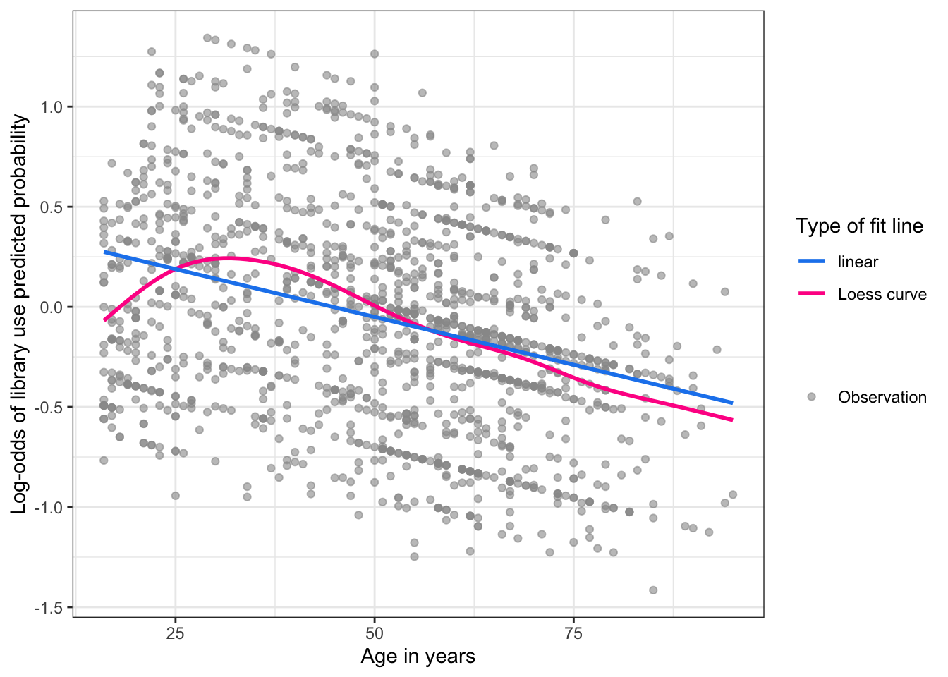
For logistic regression, the outcome variable is binary, so its relationship with another variable will never be linear. Instead of plotting the relationship of the outcome with each continuous predictor, linearity is tested by plotting the log-odds of the predicted probabilities for the outcome against each of the continuous predictors in the model. For example, are the predicted values equally accurate for people of a younger age compared to people of an older age?
R Code 10.25 : Checking linearity of the age variable for the model of library use glm10.3
#make a variable of the log-odds of the predicted values
logit_use <- log(x = glm10.3$fitted.values / (1 - glm10.3$fitted.values))

# make a small data frame with the log-odds variable and the age predictor
tbl10_lin <- tibble::tibble(logit_use, age = glm10.3$model$age)

# create a plot (Figure 10.9)
tbl10_lin  |>
  ggplot2::ggplot(
      ggplot2::aes(
          x = age,
          y = logit_use)
      ) +
  ggplot2::geom_point(
      ggplot2::aes(
          size = "Observation"
          ),
      color = "gray60",
      alpha = .6
      ) +
  ggplot2::geom_smooth(
      formula = y ~ s(x, bs = "cs"),
      method = "gam",
      se = FALSE,
      ggplot2::aes(
          color = "Loess curve")
      ) +
  ggplot2::geom_smooth(
      formula = y ~ x,
      method = lm,
      se = FALSE,
      ggplot2::aes(
          color = "linear"
          )
      ) +
  ggplot2::labs(
      x = "Age in years",
      y = "Log-odds of library use predicted probability") +
  ggplot2::scale_color_manual(
      name = "Type of fit line",
      values = c("dodgerblue2","deeppink")
      ) +
  ggplot2::scale_size_manual(
      values = 1.5,
      name = ""
      )
glm10.3
The graph shows the Loess curve close to the linear fit line with the exception of the youngest ages.
It is up to the analyst to determine whether the actual relationship is close enough to linear to meet this assumption. If the assumption is not met, this variable might be removed from analysis, transformed, or recoded.
It seems for me that there is still a problem with people 18 years old. The loess curve in Listing / Output 10.25 only gets better with people older than 25 years.
Generally I have a bad feeling with the sentence: “It is up to the analyst to determine whether the actual relationship is close enough to linear to meet this assumption.” For me there seems to much subjectivity in this approach. As I am already remarked in TODO 9.2: I have to look for tools, like statistical tests to get a more objective decision if the assumption of linearity is met.
The GVIF is similar to the VIF used for linear regression, but modified to account for the categorical outcome. It examines how well each predictor variable in the model is explained by the group of other predictor variables. If a predictor is well explained by the others, it is redundant and unnecessary. For the GVIF, often a threshold of \(GVIF^{\frac{1}{2 \times df}} < 2.5\) is used as a cutoff, with values of 2.5 or higher indicating a failed multicollinearity assumption.
R Code 10.26 : Compute GVIF
car::vif(mod = glm10.3)#> GVIF Df GVIF^(1/(2*Df))
#> age 1.254322 1 1.119965
#> sex 1.051221 1 1.025291
#> educ 1.309506 2 1.069737
#> parent 1.101618 1 1.049580
#> disabled 1.153173 1 1.073859
#> rurality 1.118617 2 1.028420
#> raceth 1.212126 2 1.049269
#> ses 1.249162 2 1.057194None of the values in the right-hand column have a value of 2.5 or higher, so there is no discernable problem with multicollinearity.
Overall, the assumption checking revealed a possible problem with age as a predictor, mostly at the youngest ages. The other assumptions were met. It might be useful to restrict the age variable to adults or to transform the age variable.
Referring to Listing / Output 9.18 residuals are the distances between the predicted value of the outcome and the true value of the outcome for each person or observation in the data set.
These values are standardized by computing z-scores for each one so that they follow a z-distribution. Standardized residuals are z-scores for the residual values. Z-scores that are greater than 1.96 or less than –1.96 are about two standard deviations or more away from the mean of a measure. In this case, they are more than two standard deviations away from the mean residual value. Very large values of standardized residuals can indicate that the predicted value for an observation is far from the true value for that observation, indicating that an examination of that observation could be useful.
Example 10.7 : Standardize residuals and check if z-scores greater than 2
R Code 10.27 : Compute and check residuals
#> # A tibble: 1 × 1
#>   max_resid
#>       <dbl>
#> 1 1.82save_data_file("chap10", tbl10.4, "tbl10.4.rds")The maximum absolute value of any standardized residual was less than 1.96, so the standardized residuals did not reveal any outliers.
R Code 10.28 : Standardized residuals for library use model
tbl10.4 |>
    # tidyr::drop_na(res_std) |>
    ggplot2::ggplot(
        ggplot2::aes(
            x = ID,
            y = res_std,
            group = "Library use"
        )
    ) +
    ggplot2::geom_jitter(
        ggplot2::aes(
            color = uses.lib
        )
    ) +
    ggplot2::labs(
        x = "Observation number",
        y = "Standarized reeisudals"
    ) +
    ggokabeito::scale_okabe_ito(
        name = "Library use",
        aesthetics = "color",
        order = c(1,3),
        alpha = .6
        )
#> Warning: Removed 174 rows containing missing values or values outside the scale range
#> (`geom_point()`).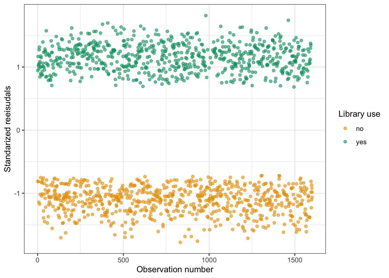
This is my reproduction of book’s Figure 10.10, using the colorblind-friendly Okabe-Ito scale. Most predicted probabilities were about one standard deviation above or below the mean predicted probability. So there were not outliers to examine.
As I already mentioned in Warning 9.1 the book mixes dfbeta & dfbetas together. But these two are different measures:
dfbetas (plural) are the standardized values, with a cutoff of \(2 / \sqrt{n}\). Because of standardization dfbetas are the recommended measure to use. - dfbeta (singular) values depend on the scale of the data.
Example 10.8 : Computing dfbeta(s)
R Code 10.29 : Computing different influence measures
## get influence statistics
infl10.3 <- stats::influence.measures(model = glm10.3)

## print influential data
glue::glue("The next two results are from 'example(influence.measure)'")
glue::glue("")
glue::glue("Print list of influential data")
which(apply(infl10.3$is.inf, 1, any))

## which observations 'are' influential
glue::glue("")
glue::glue("Which observations 'are' influential?")
summary(infl10.3)

## print all diagnostic data
glue::glue("")
glue::glue("Print a summary of all diagnostic data")
base::summary(infl10.3$infmat)
#> The next two results are from 'example(influence.measure)'
#>
#> Print list of influential data
#> named integer(0)
#>
#> Which observations 'are' influential?
#> Potentially influential observations of
#> glm(formula = uses.lib ~ age + sex + educ + parent + disabled + rurality + raceth + ses, family = binomial("logit"), data = tbl10.3, na.action = na.exclude) :
#> NONE
#> numeric(0)
#>
#> Print a summary of all diagnostic data
#> dfb.1_ dfb.age dfb.sxml
#> Min. :-0.1051922 Min. :-0.0767940 Min. :-0.039027
#> 1st Qu.:-0.0129510 1st Qu.:-0.0160893 1st Qu.:-0.023107
#> Median : 0.0000000 Median : 0.0000000 Median :-0.015882
#> Mean : 0.0001392 Mean :-0.0005355 Mean :-0.001121
#> 3rd Qu.: 0.0125725 3rd Qu.: 0.0142736 3rd Qu.: 0.024395
#> Max. : 0.1142539 Max. : 0.0825243 Max. : 0.055434
#>
#> dfb.edom dfb.et2d dfb.prnt
#> Min. :-0.1161072 Min. :-0.1179326 Min. :-0.073641
#> 1st Qu.:-0.0106307 1st Qu.:-0.0069438 1st Qu.:-0.013862
#> Median : 0.0000000 Median : 0.0000000 Median : 0.000000
#> Mean : 0.0005464 Mean : 0.0001351 Mean : 0.000333
#> 3rd Qu.: 0.0113543 3rd Qu.: 0.0068441 3rd Qu.: 0.014662
#> Max. : 0.0967673 Max. : 0.0949315 Max. : 0.069974
#>
#> dfb.dsbl dfb.rrltys dfb.rrltyr
#> Min. :-0.079962 Min. :-0.0733540 Min. :-0.0742958
#> 1st Qu.:-0.011309 1st Qu.:-0.0152557 1st Qu.:-0.0150995
#> Median : 0.000000 Median : 0.0000000 Median : 0.0000000
#> Mean :-0.000256 Mean : 0.0002054 Mean : 0.0002627
#> 3rd Qu.: 0.009065 3rd Qu.: 0.0139402 3rd Qu.: 0.0147617
#> Max. : 0.089810 Max. : 0.0741895 Max. : 0.0714801
#>
#> dfb.rN-B dfb.rN-W dfb.sslw
#> Min. :-0.0843655 Min. :-0.1059933 Min. :-9.111e-02
#> 1st Qu.:-0.0023347 1st Qu.:-0.0079223 1st Qu.:-9.360e-03
#> Median : 0.0000000 Median : 0.0000000 Median : 0.000e+00
#> Mean : 0.0003143 Mean : 0.0002498 Mean :-2.919e-05
#> 3rd Qu.: 0.0025706 3rd Qu.: 0.0083564 3rd Qu.: 8.515e-03
#> Max. : 0.0847660 Max. : 0.0939644 Max. : 9.547e-02
#>
#> dfb.ssmd dffit cov.r cook.d
#> Min. :-0.1118319 Min. :-0.17302 Min. :0.9952 Min. :0.00011
#> 1st Qu.:-0.0062815 1st Qu.:-0.09024 1st Qu.:1.0035 1st Qu.:0.00032
#> Median : 0.0000000 Median :-0.04160 Median :1.0079 Median :0.00057
#> Mean :-0.0001344 Mean :-0.00026 Mean :1.0082 Mean :0.00071
#> 3rd Qu.: 0.0073985 3rd Qu.: 0.08853 3rd Qu.:1.0127 3rd Qu.:0.00093
#> Max. : 0.1113670 Max. : 0.18890 Max. :1.0250 Max. :0.00353
#> NA's :174 NA's :174
#> hat
#> Min. :0.000000
#> 1st Qu.:0.004505
#> Median :0.007261
#> Mean :0.008120
#> 3rd Qu.:0.011625
#> Max. :0.022682
#> Generally it turned out that there are no influential values! Otherwise I would have get an output where different variable results would have be signed with an asterisk.
I had a hard time to understand the output, because the names of the variables do not conform to the name in the tibble. But after some trial and error I understood that I have to look for the variable name without vocals and add a combination of letters for the levels:
This list was confirmed after I computed dfbetas directly with Listing / Output 10.30 because I got better variable names for the results.
I added to Listing / Output 10.29 two measures provided by an additional example of the last line of the stats::lm-influence() help page (“For more”user level” examples, use example(influence.measures)“) or respectively the examples in the stats::influence.measures() help page.
R Code 10.30 : Compute dfbetas
#>   (Intercept)              age                sexmale
#>  Min.   :-0.1051922   Min.   :-0.0767940   Min.   :-0.039027
#>  1st Qu.:-0.0129510   1st Qu.:-0.0160893   1st Qu.:-0.023107
#>  Median : 0.0000000   Median : 0.0000000   Median :-0.015882
#>  Mean   : 0.0001392   Mean   :-0.0005355   Mean   :-0.001121
#>  3rd Qu.: 0.0125725   3rd Qu.: 0.0142736   3rd Qu.: 0.024395
#>  Max.   : 0.1142539   Max.   : 0.0825243   Max.   : 0.055434
#>  educFour-year degree or more educHS to 2-year degree  parentparent
#>  Min.   :-0.1161072           Min.   :-0.1179326      Min.   :-0.073641
#>  1st Qu.:-0.0106307           1st Qu.:-0.0069438      1st Qu.:-0.013862
#>  Median : 0.0000000           Median : 0.0000000      Median : 0.000000
#>  Mean   : 0.0005464           Mean   : 0.0001351      Mean   : 0.000333
#>  3rd Qu.: 0.0113543           3rd Qu.: 0.0068441      3rd Qu.: 0.014662
#>  Max.   : 0.0967673           Max.   : 0.0949315      Max.   : 0.069974
#>   disabledyes        ruralitysuburban     ruralityurban
#>  Min.   :-0.079962   Min.   :-0.0733540   Min.   :-0.0742958
#>  1st Qu.:-0.011309   1st Qu.:-0.0152557   1st Qu.:-0.0150995
#>  Median : 0.000000   Median : 0.0000000   Median : 0.0000000
#>  Mean   :-0.000256   Mean   : 0.0002054   Mean   : 0.0002627
#>  3rd Qu.: 0.009065   3rd Qu.: 0.0139402   3rd Qu.: 0.0147617
#>  Max.   : 0.089810   Max.   : 0.0741895   Max.   : 0.0714801
#>  racethNon-Hispanic Black racethNon-Hispanic White     seslow
#>  Min.   :-0.0843655       Min.   :-0.1059933       Min.   :-9.111e-02
#>  1st Qu.:-0.0023347       1st Qu.:-0.0079223       1st Qu.:-9.360e-03
#>  Median : 0.0000000       Median : 0.0000000       Median : 0.000e+00
#>  Mean   : 0.0003143       Mean   : 0.0002498       Mean   :-2.919e-05
#>  3rd Qu.: 0.0025706       3rd Qu.: 0.0083564       3rd Qu.: 8.515e-03
#>  Max.   : 0.0847660       Max.   : 0.0939644       Max.   : 9.547e-02
#>    sesmedium
#>  Min.   :-0.1118319
#>  1st Qu.:-0.0062815
#>  Median : 0.0000000
#>  Mean   :-0.0001344
#>  3rd Qu.: 0.0073985
#> Max. : 0.1113670dfbetas
Besides the better variable names it also turned out the in Listing / Output 10.29 the results are dfbetas and not dfbeta as I have computed in Listing / Output 10.31 to see the differences.
R Code 10.31 : Compute dfbeta
#>   (Intercept)              age                sexmale
#>  Min.   :-4.116e-02   Min.   :-2.908e-04   Min.   :-0.0050592
#>  1st Qu.:-5.068e-03   1st Qu.:-6.093e-05   1st Qu.:-0.0029956
#>  Median : 0.000e+00   Median : 0.000e+00   Median :-0.0020589
#>  Mean   : 5.456e-05   Mean   :-2.031e-06   Mean   :-0.0001456
#>  3rd Qu.: 4.920e-03   3rd Qu.: 5.405e-05   3rd Qu.: 0.0031625
#>  Max.   : 4.471e-02   Max.   : 3.124e-04   Max.   : 0.0071843
#>  educFour-year degree or more educHS to 2-year degree  parentparent
#>  Min.   :-0.0284321           Min.   :-2.685e-02      Min.   :-1.148e-02
#>  1st Qu.:-0.0026041           1st Qu.:-1.582e-03      1st Qu.:-2.162e-03
#>  Median : 0.0000000           Median : 0.000e+00      Median : 0.000e+00
#>  Mean   : 0.0001341           Mean   : 3.084e-05      Mean   : 5.204e-05
#>  3rd Qu.: 0.0027817           3rd Qu.: 1.559e-03      3rd Qu.: 2.287e-03
#>  Max.   : 0.0237047           Max.   : 2.162e-02      Max.   : 1.091e-02
#>   disabledyes         ruralitysuburban     ruralityurban
#>  Min.   :-1.479e-02   Min.   :-1.196e-02   Min.   :-1.231e-02
#>  1st Qu.:-2.092e-03   1st Qu.:-2.488e-03   1st Qu.:-2.503e-03
#>  Median : 0.000e+00   Median : 0.000e+00   Median : 0.000e+00
#>  Mean   :-4.745e-05   Mean   : 3.356e-05   Mean   : 4.363e-05
#>  3rd Qu.: 1.676e-03   3rd Qu.: 2.274e-03   3rd Qu.: 2.448e-03
#>  Max.   : 1.661e-02   Max.   : 1.210e-02   Max.   : 1.185e-02
#>  racethNon-Hispanic Black racethNon-Hispanic White     seslow
#>  Min.   :-2.185e-02       Min.   :-2.160e-02       Min.   :-2.612e-02
#>  1st Qu.:-6.046e-04       1st Qu.:-1.616e-03       1st Qu.:-2.683e-03
#>  Median : 0.000e+00       Median : 0.000e+00       Median : 0.000e+00
#>  Mean   : 8.155e-05       Mean   : 5.104e-05       Mean   :-8.383e-06
#>  3rd Qu.: 6.658e-04       3rd Qu.: 1.704e-03       3rd Qu.: 2.441e-03
#>  Max.   : 2.195e-02       Max.   : 1.916e-02       Max.   : 2.736e-02
#>    sesmedium
#>  Min.   :-2.538e-02
#>  1st Qu.:-1.426e-03
#>  Median : 0.000e+00
#>  Mean   :-3.055e-05
#>  3rd Qu.: 1.679e-03
#> Max. : 2.527e-02dfbeta
These dfbeta values are quite different to the dfbetas.
I am not sure if the dfbeta values are — beside of linear models computed with stats::lm() — also valid for generalized linear models, computed with stats::glm(). My doubts are nurtured on the fact that in the help file all computed dfbeta and dfbetas require a method of class lm. This is in contrast to Cook’s D where a method for both classes lm and glm exists.
See also the explanation of the argument ìnfl`:
influence structure as returned by
lm.influenceorinfluence(the latter only for the glm method of rstudent and cooks.distance).
Cook’s Distance, is computed in a similar way to dfbeta(s) — each observation is removed and the model is re-estimated without it. Cook’s D then combines the differences between the models with and without an observation for all the parameters together instead of one at a time like the dfbeta(s). A high Cook’s D would indicate that removing the observation made a big difference and therefore it might be considered influential.
R Code 10.32 : Compute Cook’s D
tibble::tibble(infl_cooks_d = cooks.distance(glm10.3)) |>
    tidyr::drop_na() |>
    dplyr::filter(infl_cooks_d > 4 / dplyr::n())
#> # A tibble: 6 × 1
#> infl_cooks_d
#> <dbl>
#> 1 0.00301
#> 2 0.00298
#> 3 0.00353
#> 4 0.00280
#> 5 0.00327
#> 6 0.00282Depending if I compute it with NA’s or without NA’s I got 12 or six influential values. This is in contrast to Listing / Output 10.29, where I couldn’t detect any influential values.
But I cannot see which row in the data these six values belong. I think that would be necessary to inspect and/or delete these values.
Leverage is the influence that the observed value of the outcome has on the predicted value of the outcome. Leverage values range between 0 and 1. To determine which leverage values indicate influential observations, a cutoff of \(\frac{2p}{n}\)is often used. In this case, we have 13 parameters, so the cutoff is \(\frac{2 \times 13}{1427}= 0.01822004\)
R Code 10.33 : Compute leverage (hat values)
#> # A tibble: 95 × 1
#>       hat
#>     <dbl>
#>  1 0.0184
#>  2 0.0190
#>  3 0.0185
#>  4 0.0184
#>  5 0.0164
#>  6 0.0176
#>  7 0.0219
#>  8 0.0180
#>  9 0.0205
#> 10 0.0198
#> # ℹ 85 more rowsInstead of 35 values I got 95 influential values. The reason for the difference is that there are 1601 records and not 1427 as calculated in the book.
But all in all I still think that both results 35 and 95 are wrong, because the variable infl10.3$is.inf has not even a single TRUE value for any measures as already shown in Listing / Output 10.29.
TODO: Look for other tutorials how to compute influential values
I think that there are several reasons why the computation of the influential values in the book has some inaccuracies:
dfbeta and dfbetas. In the book both measures are treated the same, but there is a difference. (BTW: Both measures are written without a dash as is the case in the book.)lm-measures work the same with glm. In the help file there are several hints that there exist differences.stats::influential.measures() as explained in the examples of the help files does not show any TRUEs for the diagnosis variable is.inf.There are many tutorials explaining how to work with outliers and influential values. But these texts — often buried in textbooks — are complex. I need to dedicate some time to read and to try out their data examples. But from the big importance that this subject has, I will explores some of these tutorials.
Remark 10.2. : Difference between outliers and influential points
There was no good explication in the book about the difference between outliers and influential values. (See for the clarification in section 12.6 of Introductory Statistics, (Illowsky and Dean 2011, 541)).
Outliers are observed data points that are far from the least squares line. They have large “errors”, where the “error” or residual is the vertical distance from the line to the point.
Besides outliers, a sample may contain one or a few points that are called influential points. Influential points are observed data points that are far from the other observed data points in the horizontal direction. These points may have a big effect on the slope of the regression line. To begin to identify an influential point, you can remove it from the data set and see if the slope of the regression line is changed significantly.
R Code 10.34 : Anscombe’s Quartet of ‘Identical’ Simple Linear Regressions
## Now, do what you should have done in the first place: PLOTS
ff <- y ~ x
mods <- setNames(as.list(1:4), paste0("lm", 1:4))
for(i in 1:4) {
    ff[2:3] <- lapply(paste0(c("y", "x"), i), as.name)
    mods[[i]] <- lmi <- lm(ff, data = anscombe)
}

op <-
    par(
        mfrow = c(2, 2),
        mar = 0.1 + c(4, 4, 1, 1),
        oma =  c(0, 0, 2, 0)
    )
for (i in 1:4) {
    ff[2:3] <- lapply(paste0(c("y", "x"), i), as.name)
    plot(
        ff,
        data = anscombe,
        col = "red",
        pch = 21,
        bg = "orange",
        cex = 1.2,
        xlim = c(3, 19),
        ylim = c(3, 13)
    )
    abline(mods[[i]], col = "blue")
}
mtext("Anscombe's 4 Regression data sets",
      outer = TRUE,
      cex = 1.5)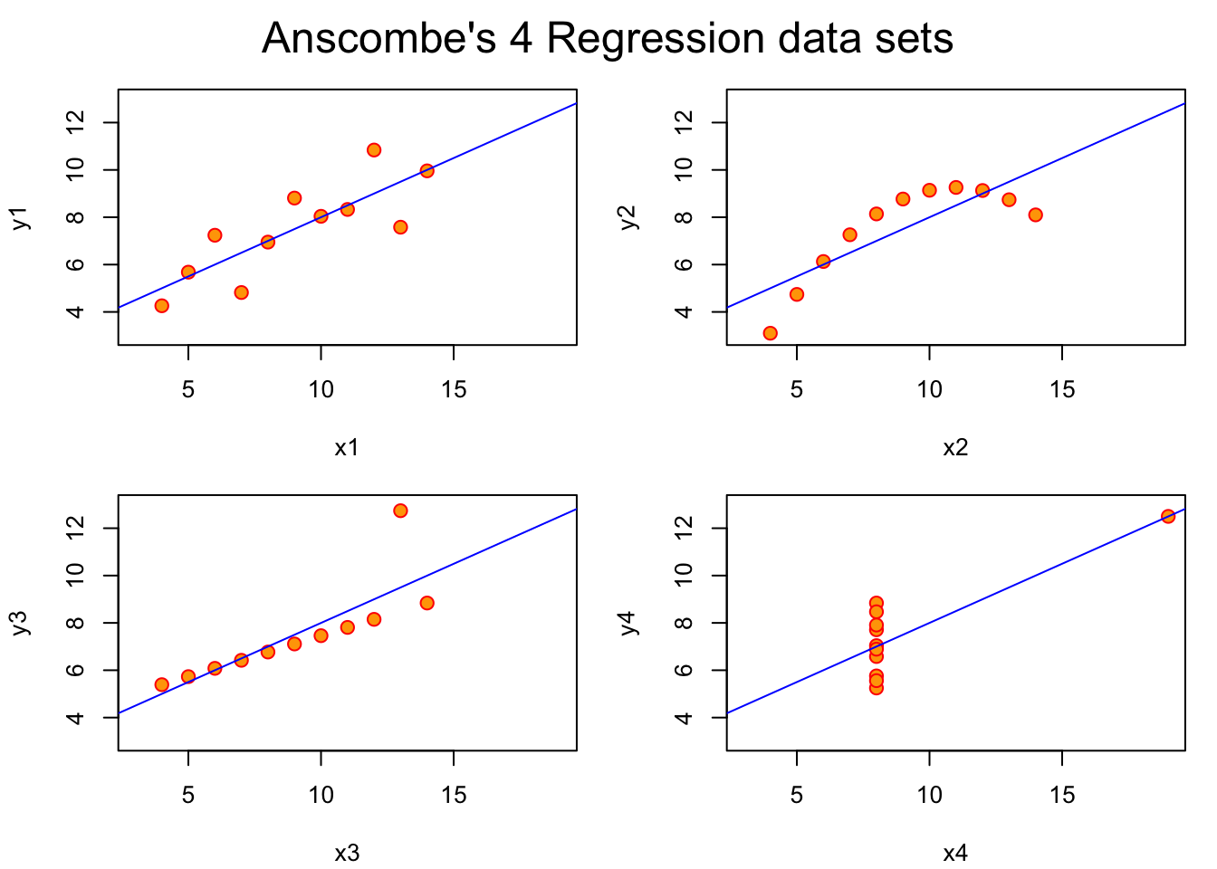
Listing / Output 10.34 shows the difference between outlier and influential point very clearly:
Logistic regression models are useful not only for examining relationships between predictors and binary outcomes, but also for predicting probabilities for hypothetical or new cases that are not in the data frame.
R Code 10.35 : Using the model to predict probabilities for observations that are outside the data set
# make a new data frame containing the observations of interest
glm10.3_example <- tibble::tibble(age = c(35, 65, 68),
                         sex = c("male", "female", "male"),
                         educ = c("Four-year degree or more",
                                  "Four-year degree or more",
                                  "Four-year degree or more"),
                         disabled = c("no", "no", "no"),
                         parent = c("not parent", "parent", "parent"),
                         rurality = c("rural", "rural", "rural"),
                         raceth = c("Non-Hispanic White",
                                    "Non-Hispanic White",
                                    "Non-Hispanic White"),
                         ses = c("low", "medium", "medium"))

# use the new data frame to predict
predictions <- predict(object = glm10.3, newdata = glm10.3_example,
                       type = "response")
predictions
#> 1 2 3
#> 0.5135547 0.6466977 0.4648331An interaction term examines how two (or more) variables might work together to influence an outcome. A possible interaction between sex and parental status can be included in the logistic regression model by adding a term, \(+ sex \times parent\), to the formula. When an interaction is included in a model, it is customary to also include the interacting variables separately. In a model with interaction terms, the terms that are not part of the interaction are called main effects.
R Code 10.36 : Computing interaction parental status and sex
# estimate the library use model for interaction term and print results
glm10.4 <- glm(formula = uses.lib ~ age + sex + educ + parent +
                         disabled + rurality + ses + raceth + sex*parent,
             data = tbl10.4,
             family = binomial("logit")
             )

odds.n.ends::odds.n.ends(mod = glm10.4)
#> Waiting for profiling to be done...#> $`Logistic regression model significance`
#> Chi-squared d.f. p
#> 96.296 13 <.001
#>
#> $`Contingency tables (model fit): frequency predicted`
#> Number observed
#> Number predicted 1 0 Sum
#> 1 383 264 647
#> 0 313 467 780
#> Sum 696 731 1427
#>
#> $`Count R-squared (model fit): percent correctly predicted`
#> [1] 59.56552
#>
#> $`Model sensitivity`
#> [1] 0.5502874
#>
#> $`Model specificity`
#> [1] 0.6388509
#>
#> $`Predictor odds ratios and 95% CI`
#> OR 2.5 % 97.5 %
#> (Intercept) 1.3896208 0.7106390 2.7205274
#> age 0.9894621 0.9830350 0.9958813
#> sexmale 0.4518131 0.3500795 0.5816044
#> educFour-year degree or more 1.9341335 1.2770482 2.9441143
#> educHS to 2-year degree 1.1558031 0.7862126 1.7074900
#> parentparent 1.0553800 0.7182384 1.5579958
#> disabledyes 0.7939236 0.5785547 1.0867415
#> ruralitysuburban 1.1796693 0.8937225 1.5575559
#> ruralityurban 1.2198083 0.9199887 1.6180430
#> seslow 0.9509862 0.5828701 1.5483108
#> sesmedium 0.8534710 0.5788626 1.2539095
#> racethNon-Hispanic Black 1.5599911 1.0060581 2.4253682
#> racethNon-Hispanic White 1.3110430 0.9283916 1.8568026
#> sexmale:parentparent 1.3855389 0.8300643 2.3074929glm10.4 with interaction parental status and sex
Write the null and alternate hypotheses:
Compute the test statistic.
The test statistic is \(χ^2 = 96.30\) with 13 degrees of freedom.
Review and interpret the test statistics: Calculate the probability that your test statistic is at least as big as it is if there is no relationship (i.e., the null is true).
The p-value is less than .001.
Conclude and write report.
The null hypothesis is rejected. The model including age, sex, education, parent status, disability status, rurality, SES, race-ethnicity, and an interaction between sex and parent status is useful in explaining library use [\(χ^2(13) = 96.30; p < .001\)].
Thee is nothing new in this section.
Given that the interaction term was not statistically significant and the model violated the linearity assumption, it seems preferable to report the previous model without the interaction term as the final model. However, there is a statistical test that can be used to determine whether a larger model is statistically significantly better than a smaller model. The test is called the likelihood ratio test.
The likelihood ratio (LR) test compares two nested models where one model includes a subset of the variables in the other model. For example, the simple logistic regression model with age as the only predictor could be compared statistically to any of the larger models because they all have the age variable in them. The small model is nested in each of the larger models. In addition, the larger model without the interaction could be compared to the model with the interaction term. Models where the variables of one are completely different from the variables of the other cannot be compared with this test.
The idea behind the LR test is to determine if the additional variables in a model make the model better enough to warrant the complexity of adding more variables to the model.
Write the null and alternate hypotheses:
Compute the test statistic.
The {lmtest} package (Section A.45) has the lrtest() function, which can be used to compare two nested models. The LR test computes the difference between the log-likelihoods for the two models and multiplies this by 2; the result has a chi-squared distribution.
R Code 10.37 : Likelihood ratio test
lmtest::lrtest(object = glm10.3, glm10.4)#> Likelihood ratio test
#>
#> Model 1: uses.lib ~ age + sex + educ + parent + disabled + rurality +
#> raceth + ses
#> Model 2: uses.lib ~ age + sex + educ + parent + disabled + rurality +
#> ses + raceth + sex * parent
#> #Df LogLik Df Chisq Pr(>Chisq)
#> 1 13 -941.32
#> 2 14 -940.54 1 1.5599 0.2117The output from lmtest::lrtest() shows the test statistic is \(χ^2 = 1.56\).
Review and interpret the test statistics: Calculate the probability that your test statistic is at least as big as it is if there is no relationship (i.e., the null is true).
The test statistic of \(χ^2 = 1.56\) had a p-value of .21.
Conclude and write report.
When the larger model is not statistically significantly better, then use of the smaller model to aid in interpretation is preferred. The more complex a model becomes, the more difficult it is to interpret. Generally speaking, parsimony is preferable. However, there are exceptions to this, such as when the larger model has variables in it that have been consistently related to the outcome in other research or are important to understanding the outcome for some other reason.
Example 10.9 : Forest plot for reporting odds ratios
R Code 10.38 : Forest plot for reporting odds ratios (Version 1)
# get odds ratio table from glm10.3
# not [4] as in the book, but [6]
df10.3_odds <- data.frame(
    odds.n.ends::odds.n.ends(mod = glm10.3)[6]
)
#> Waiting for profiling to be done...# change variable names for easier use
names(df10.3_odds) <- c("OR", "lower", "upper")
# make row names a variable
tbl10.3_odds <- df10.3_odds |>
tibble::rownames_to_column(var = "variable")
# forest plot of odds ratios from glm10.3 (Figure 10.15)
tbl10.3_odds |>
ggplot2::ggplot(
ggplot2::aes(
x = variable,
y = OR,
ymin = lower,
ymax = upper)
) +
ggplot2::geom_pointrange(color = "#7463AC") +
ggplot2::geom_hline(
yintercept = 1,
lty = 2,
color = "deeppink",
linewidth = 1) +
ggplot2::coord_flip() +
ggplot2::labs(x = "Variable from library use model", y = "Odds ratio (95% CI)") 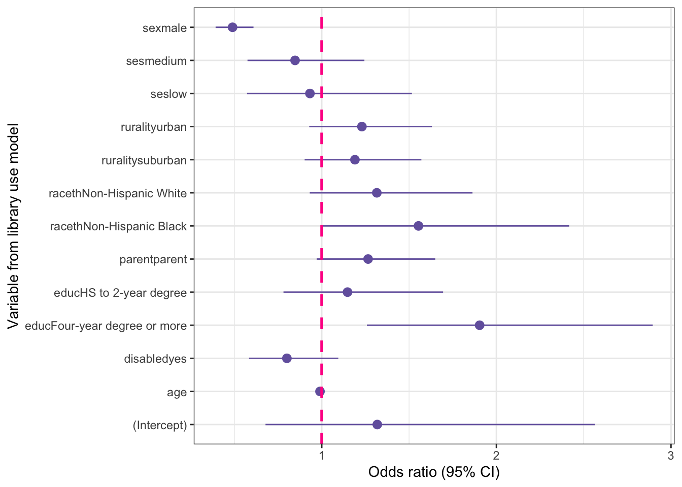
R Code 10.39 : Forest plot for reporting odds ratios (Version 2)
# clean variable names for graph
tbl10.3_odds_clean <- tbl10.3_odds |>
  dplyr::mutate(
      variable = dplyr::recode(.x = variable,
           "sexmale" = "Male",
           "ruralityurban" = "Urban residence",
           "ruralitysuburban" = "Suburban residence",
           "parentparent" = "Parent",
           "educHS to 2-year degree" = "HS to 2-year degree",
           "educFour-year degree or more" = "Four-year degree or more",
           "disabledyes" = "Disabled",
           "age" = "Age",
           "seslow" = "Low socioeconomic status",
           "sesmedium" = "Medium socioeconomic status",
           "racethNon-Hispanic White" = "Non-Hispanic White",
           "racethNon-Hispanic Black" = "Non-Hispanic Black",
           "(Intercept)" = "Intercept")
      )

# modify graph to include clean variable names (Figure 10.16)
# change scale of y-axis (flipped) to log scale for visualization
tbl10.3_odds_clean |>
  ggplot2::ggplot(
      ggplot2::aes(
          x = variable,
          y = OR,
          ymin = lower,
          ymax = upper)) +
  ggplot2::geom_pointrange(color = "#7463AC") +
  ggplot2::geom_hline(
      yintercept = 1,
      lty = 2,
      color = "deeppink",
      linewidth = 1) +
  ggplot2::scale_y_log10(
      breaks = c(0.1, 0.2, 0.5, 1.0, 2.0, 5.0, 10),
                minor_breaks = NULL) +
  ggplot2::coord_flip() +
  ggplot2::labs(
      x = "Variable from library use model",
y = "Odds ratio (95% CI)") 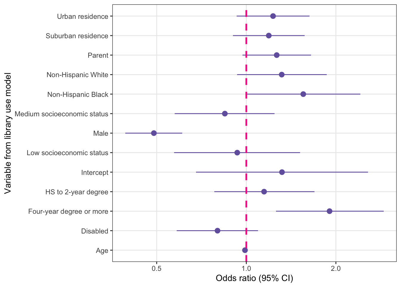
R Code 10.40 : Forest plot for reporting odds ratios (Final version)
tbl10.3_odds_clean |>
  ggplot2::ggplot(
      ggplot2::aes(x =
               reorder(variable, OR),
               y = OR,
               ymin = lower,
               ymax = upper)) +
  ggplot2::geom_pointrange(color = "#7463AC") +
  ggplot2::geom_hline(
      yintercept = 1,
      lty = 2,
      color = "deeppink",
      linewidth = 1) +
  ggplot2::scale_y_log10(
      breaks = c(0.1, 0.2, 0.5, 1.0, 2.0, 5.0, 10),
      minor_breaks = NULL) +
  ggplot2::coord_flip() +
  ggplot2::labs(
      x = "Variable from library use model",
      y = "Odds ratio (95% CI)")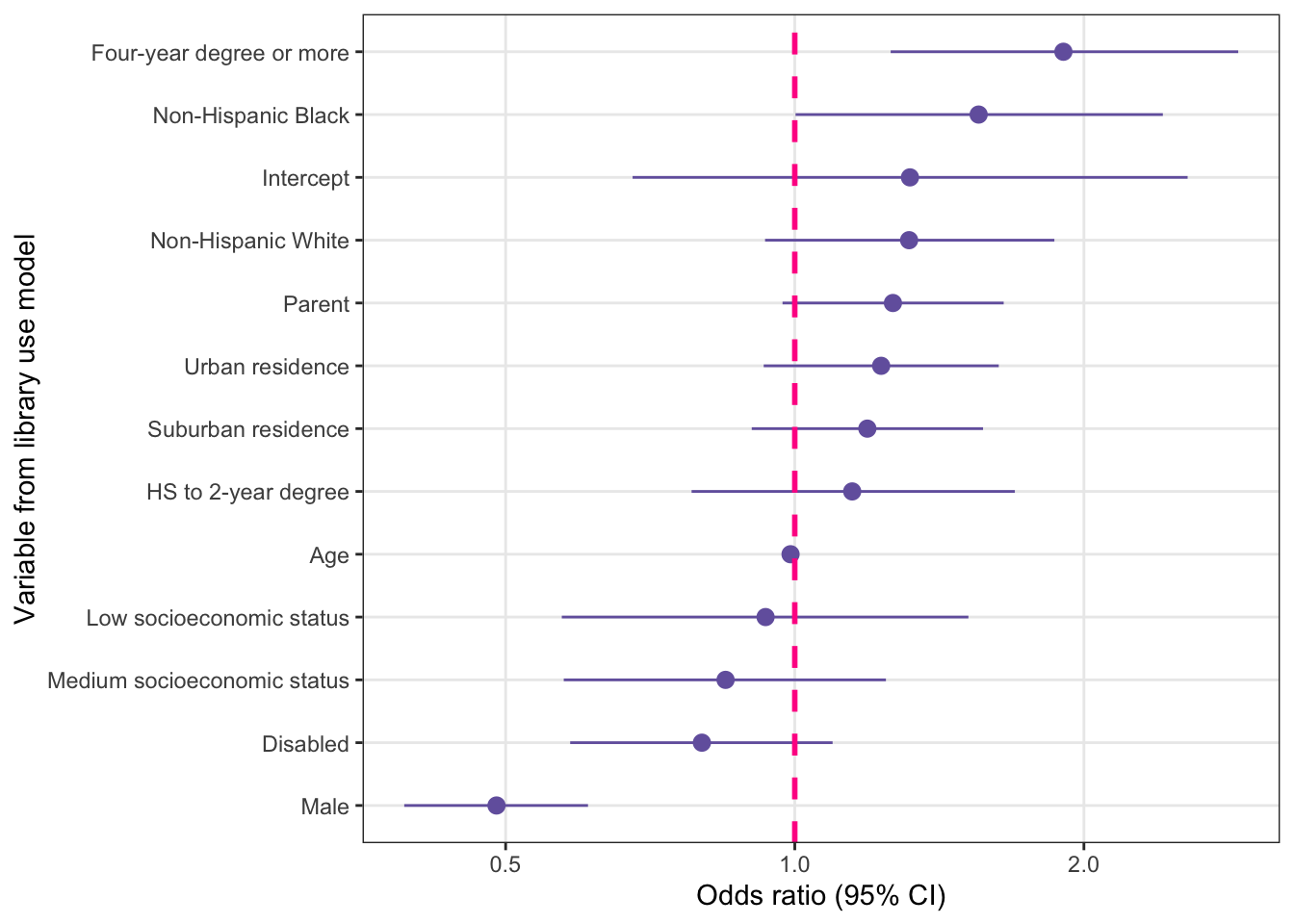
| term | definition |
|---|---|
| Adjusted-count-R2 | Adjusted count R-squared is a measure of model fit for binary logistic regression that adjusts the percent correctly predicted (or count R-squared) by the model for the number of people in the largest outcome category. (SwR, Glossary) |
| B-Spline | The term "spline" refers to a wide class of basis functions that are used in applications requiring data interpolation and/or smoothing. Splines are special function defined piecewise by polynomials, it results to a smooth function built out of smaller, component functions. In interpolating problems, spline interpolation is often preferred to polynomial interpolation because it yields similar results, even when using low degree polynomials, while avoiding big numbers and the problem of oscillation at the edges of intervals of higher degrees. The term "spline" comes from the flexible [spline](https://en.wikipedia.org/wiki/Flat_spline) devices used by shipbuilders and draftsmen to draw smooth shapes. They used a long, thin piece of wood or metal that could be anchored in a few places in order to aid drawing curves. There are many types of splines, especially the common-place 'B-splines': The 'B' stands for 'basis,' which just means 'component.' B-splines build up wiggly functions from simpler less-wiggly components. Those components are called basis functions. B-splines force you to make a number of choices t |
| Confidence Interval | A range of values, calculated from the sample observations, that is believed, with a particular probability, to contain the true parameter value. (Cambridge Dictionary of Statistics, 4th ed., p.98) |
| Cook’s D | Cook’s distance (often abbreviated Cook’s D) is used in Regression Analysis to find influential outliers in a set of predictor variables. IIt is a way to identify points that negatively affect the regression model. ([Statistics How To](https://www.statisticshowto.com/cooks-distance/)) |
| Count-R-squared | Count R-squared, or percent correctly predicted, is a measure of model fit for a logistic regression model that is the proportion of the outcome values that were correctly predicted out of all observations modeled. (SwR, Glossary) |
| Cumulative Distribution Function | A cumulative distribution function (CDF) tells us the probability that a random variable takes on a value less than or equal to x. (<a href="https://www.statology.org/cdf-vs-pdf/">Statology</a>) It sums all parts of the distribution, replacing a lot of calculus work. The CDF takes in a value and returns the probability of getting that value or lower. (BF, Chap.13) A CDF is a hypothetical model of a distribution, the ECDF models empirical (i.e. observed) data. (<a href="https://www.statisticshowto.com/empirical-distribution-function/">Statistics How To</a>) |
| dfbeta | dfbeta are effects on coefficients of deleting each observation in turn. ("Companion to Applied Regression", car package, help file) |
| dfbetas | dfbetas are effect on coefficients of deleting each observation in turn, standardized by a deleted estimate of the coefficient standard error ("Companion to Applied Regression", car package, help file) |
| Digital Divide | The term "digital divide" refers to the gap between individuals, households, businesses and geographic areas at different socio-economic levels with regard to their opportunities to access information and communication technologies (ICTs). (<a href= "https://www.oecd-ilibrary.org/science-and-technology/understanding-the-digital-divide_236405667766">OECD Library</a>) |
| EDA | Explorative Data Analysis is an approach of analyzing data sets to summarize their main characteristics, often using statistical graphics and other data visualization methods. A statistical model can be used or not, but primarily EDA is for seeing what the data can tell us beyond the formal modeling and thereby contrasts traditional hypothesis testing. (<a href="https://en.wikipedia.org/wiki/Exploratory_data_analysis">Wikipedia</a>) |
| GLM | A generalized linear model (GLM) is a flexible generalization of ordinary linear regression. The GLM generalizes linear regression by allowing the linear model to be related to the response variable via a link function and by allowing the magnitude of the variance of each measurement to be a function of its predicted value. (<a href="https://en.wikipedia.org/w/index.php?title=Generalized_linear_model&oldid=1175448680">Wikipedia</a>). the binary logistic regression model is one example of a generalized linear model. (SwR, Glossary) |
| Goodness-of-fit | The chi-squared goodness-of-fit test is used for comparing the values of a single categorical variable to values from a hypothesized or population variable. The goodness-of-fit test is often used when trying to determine if a sample is a good representation of the population. (SwR, Chap 5) |
| GVIF | The generalized variance inflation factor (GVIF) is a generalized version of the variance inflation factor (VIF) that is used to identify problems with multicollinearity; the GVIF is used in binary logistic regression. (SwR, Glossary) |
| Influential Observation | An influential observation is an observation that changes the slope of a regression line. (SwR, Glossary) Influential points are observed data points that are far from the other observed data points in the horizontal direction. These points may have a big effect on the slope of the regression line. To begin to identify an influential point, you can remove it from the data set and see if the slope of the regression line is changed significantly. (<a href= "https://openstax.org/books/introductory-statistics/pages/12-6-outliers">Introductory Statistics 12.6</a>) |
| Likelihood-ratio | The likelihood ratio test is a test that compares two nested binary logistic regression models to determine which is a better fit to the data; the difference between two log-likelihoods follows a chi-squared distribution with a significant result indicating the larger model is a better fitting model. (SwR, Glossary) |
| Linear Regression | Linear regression is used to predict the value of an outcome variable Y based on one or more input predictor variables X. The aim is to establish a linear relationship (a mathematical formula) between the predictor variable(s) and the response variable, so that, we can use this formula to estimate the value of the response Y, when only the predictors (Xs) values are known. ([r-statistics.co](https://r-statistics.co/Linear-Regression.html)) (Chap.4) |
| Linearity | Linearity is the assumption of some statistical models that requires the outcome, or transformed outcome, to have a linear relationship with numeric predictors, where linear relationships are relationships that are evenly distributed around a line. (SwR, Glossary) |
| Logit Transformations | Logit transformations are transformations that takes the log value of p/(1-p); this transformation is often used to normalize percentage data and is used in the logistic model to transform the outcome. (SwR, Glossary) |
| Odds Ratio | Odds is usually defined in statistics as the probability an event will occur divided by the probability that it will not occur. An odds ratio (OR) is a measure of association between a certain property A and a second property B in a population. Specifically, it tells you how the presence or absence of property A has an effect on the presence or absence of property B. (<a href="https://www.statisticshowto.com/probability-and-statistics/probability-main-index/odds-ratio/">Statistics How To</a>). An odds ratio is a ratio of two ratios. They quantify the strength of the relationship between two conditions. They indicate how likely an outcome is to occur in one context relative to another. (<a href="https://statisticsbyjim.com/probability/odds-ratio/">Statistics by Jim</a>) |
| Outcome | Outcome is the variable being explained or predicted by a model; in linear and logistic regression, the outcome variable is on the left-hand side of the equal sign. (SwR, Glossary) |
| Outliers | Outliers are observations with unusual values. (SwR, Glossary). Outliers are observed data points that are far from the least squares line. They have large "errors", where the "error" or residual is the vertical distance from the line to the point. (<a href= "https://openstax.org/books/introductory-statistics/pages/12-6-outliers">Introductory Statistics 12.6</a>) |
| p-value | The p-value is the probability that the test statistic is at least as big as it is under the null hypothesis (SwR, Glossary) |
| A probability density function (PDF) describes a probability distribution for a random, continuous variable. Use a probability density function to find the chances that the value of a random variable will occur within a range of values that you specify. More specifically, a PDF is a function where its integral for an interval provides the probability of a value occurring in that interval. (<a href="https://statisticsbyjim.com/probability/probability-density-function/">Statistics By Jim</a>) | |
| Predictor Variable | Predictor variable -- also known sometimes as the independent or explanatory variable -- is the counterpart to the response or dependent variable. Predictor variables are used to make predictions for dependent variables. ([DeepAI](https://deepai.org/machine-learning-glossary-and-terms/predictor-variable), [MiniTab](https://support.minitab.com/en-us/minitab/21/help-and-how-to/statistical-modeling/regression/supporting-topics/basics/what-are-response-and-predictor-variables/)) |
| QRP | Questionable Research Practice (QRP) is a research practice that introduces bias, usually in pursuit of statistical significance; an example of such practices might be dropping or recoding values or variables solely to improve a model fit statistic. (SwR, GLossary) |
| Quantile | Quantiles are cut points dividing the range of a probability distribution into continuous intervals with equal probabilities (<a href="https://en.wikipedia.org/wiki/Quantile">Wikipedia</a>) |
| Residually | Residuals are the differences between the observed values and the predicted values. (SwR, Glossary) |
| Sensitivity | The true positive rate (one minus the false negative rate), is referred to as sensitivity, recall, or probability of detection. (Bayesian Thinking, Chap.1). But also the percentage of “yes” values or 1s a logistic regression model got right. (SwR, Glossary) |
| Sigmoid | A sigmoid function is any mathematical function whose graph has a characteristic S-shaped curve or sigmoid curve. (<a href="https://en.wikipedia.org/wiki/Sigmoid_function">Wikipedia</a>) |
| Specificity | The true negative rate (one minus the false positive rate), is referred to as specificity. (Bayesian Thinking, Chap.1) But also the percentage of “no” values or 0s a logistic regression model predicted correctly. (SwR, Glossary) |
| Standard Deviation | The standard deviation is a measure of the amount of variation or dispersion of a set of values. A low standard deviation indicates that the values tend to be close to the mean (also called the expected value) of the set, while a high standard deviation indicates that the values are spread out over a wider range. The standard deviation is the square root of its variance. A useful property of the standard deviation is that, unlike the variance, it is expressed in the same unit as the data. Standard deviation may be abbreviated SD, and is most commonly represented in mathematical texts and equations by the lower case Greek letter $\sigma$ (sigma), for the population standard deviation, or the Latin letter $s$ for the sample standard deviation. ([Wikipedia](https://en.wikipedia.org/wiki/Standard_deviation)) |
| Standard Error | The standard error (SE) of a statistic is the standard deviation of its [sampling distribution]. If the statistic is the sample mean, it is called the standard error of the mean (SEM). (<a href="https://en.wikipedia.org/wiki/Standard_error">Wikipedia</a>) The standard error is a measure of variability that estimates how much variability there is in a population based on the variability in the sample and the size of the sample. (SwR, Glossary) |
| VIF | The variance inflation factor (VIF) is a statistic for determining whether there is problematic multicollinearity in a linear regression model. (SwR, Glossary) |
| Wald | Wald test is the statistical test for comparing the value of the coefficient in linear or logistic regression to the hypothesized value of zero; the form is similar to a one-sample t-test, although some Wald tests use a t-statistic and others use a z-statistic as the test statistic. (SwR, Glossary) |
| Z-score | A z-score (also called a standard score) gives you an idea of how far from the mean a data point is. But more technically it’s a measure of how many standard deviations below or above the population mean a raw score is. (<a href="https://www.statisticshowto.com/probability-and-statistics/z-score/#Whatisazscore">StatisticsHowTo</a>) |
Session Info
sessioninfo::session_info()#> ─ Session info ───────────────────────────────────────────────────────────────
#> setting value
#> version R version 4.4.2 (2024-10-31)
#> os macOS Sequoia 15.1
#> system x86_64, darwin20
#> ui X11
#> language (EN)
#> collate en_US.UTF-8
#> ctype en_US.UTF-8
#> tz Europe/Vienna
#> date 2024-11-13
#> pandoc 3.5 @ /usr/local/bin/ (via rmarkdown)
#>
#> ─ Packages ───────────────────────────────────────────────────────────────────
#> package * version date (UTC) lib source
#> abind 1.4-8 2024-09-12 [2] CRAN (R 4.4.1)
#> backports 1.5.0 2024-05-23 [2] CRAN (R 4.4.0)
#> base64enc 0.1-3 2015-07-28 [2] CRAN (R 4.4.0)
#> boot 1.3-31 2024-08-28 [2] CRAN (R 4.4.2)
#> broom 1.0.7 2024-09-26 [2] CRAN (R 4.4.1)
#> broom.mixed 0.2.9.6 2024-10-15 [2] CRAN (R 4.4.1)
#> car 3.1-3 2024-09-27 [2] CRAN (R 4.4.1)
#> carData 3.0-5 2022-01-06 [2] CRAN (R 4.4.0)
#> cellranger 1.1.0 2016-07-27 [2] CRAN (R 4.4.0)
#> checkmate 2.3.2 2024-07-29 [2] CRAN (R 4.4.1)
#> class 7.3-22 2023-05-03 [2] CRAN (R 4.4.2)
#> cli 3.6.3 2024-06-21 [2] CRAN (R 4.4.1)
#> cluster 2.1.6 2023-12-01 [2] CRAN (R 4.4.2)
#> cmprsk 2.2-12 2024-05-19 [2] CRAN (R 4.4.0)
#> coda 0.19-4.1 2024-01-31 [2] CRAN (R 4.4.0)
#> codetools 0.2-20 2024-03-31 [2] CRAN (R 4.4.2)
#> colorspace 2.1-1 2024-07-26 [2] CRAN (R 4.4.0)
#> commonmark 1.9.2 2024-10-04 [2] CRAN (R 4.4.1)
#> crayon 1.5.3 2024-06-20 [2] CRAN (R 4.4.0)
#> curl 6.0.0 2024-11-05 [2] CRAN (R 4.4.1)
#> data.table 1.16.2 2024-10-10 [2] CRAN (R 4.4.1)
#> datawizard 0.13.0 2024-10-05 [2] CRAN (R 4.4.1)
#> DescTools 0.99.58 2024-11-08 [2] CRAN (R 4.4.1)
#> digest 0.6.37 2024-08-19 [2] CRAN (R 4.4.1)
#> dplyr 1.1.4 2023-11-17 [2] CRAN (R 4.4.0)
#> e1071 1.7-16 2024-09-16 [2] CRAN (R 4.4.1)
#> emmeans 1.10.5 2024-10-14 [2] CRAN (R 4.4.1)
#> Epi 2.56 2024-10-01 [2] CRAN (R 4.4.1)
#> epitools 0.5-10.1 2020-03-22 [2] CRAN (R 4.4.0)
#> estimability 1.5.1 2024-05-12 [2] CRAN (R 4.4.0)
#> etm 1.1.1 2020-09-08 [2] CRAN (R 4.4.0)
#> evaluate 1.0.1 2024-10-10 [2] CRAN (R 4.4.1)
#> Exact 3.3 2024-07-21 [2] CRAN (R 4.4.0)
#> expm 1.0-0 2024-08-19 [2] CRAN (R 4.4.1)
#> fansi 1.0.6 2023-12-08 [2] CRAN (R 4.4.0)
#> farver 2.1.2 2024-05-13 [2] CRAN (R 4.4.0)
#> fastmap 1.2.0 2024-05-15 [2] CRAN (R 4.4.0)
#> forcats 1.0.0 2023-01-29 [2] CRAN (R 4.4.0)
#> foreign 0.8-87 2024-06-26 [2] CRAN (R 4.4.2)
#> Formula 1.2-5 2023-02-24 [2] CRAN (R 4.4.0)
#> furrr 0.3.1 2022-08-15 [2] CRAN (R 4.4.0)
#> future 1.34.0 2024-07-29 [2] CRAN (R 4.4.0)
#> generics 0.1.3 2022-07-05 [2] CRAN (R 4.4.0)
#> ggformula 0.12.0 2023-11-09 [2] CRAN (R 4.4.0)
#> ggokabeito 0.1.0 2021-10-18 [2] CRAN (R 4.4.0)
#> ggplot2 3.5.1 2024-04-23 [2] CRAN (R 4.4.0)
#> ggridges 0.5.6 2024-01-23 [2] CRAN (R 4.4.0)
#> gld 2.6.6 2022-10-23 [2] CRAN (R 4.4.0)
#> globals 0.16.3 2024-03-08 [2] CRAN (R 4.4.0)
#> glossary * 1.0.0.9003 2024-08-05 [2] Github (debruine/glossary@05e4a61)
#> glue 1.8.0 2024-09-30 [2] CRAN (R 4.4.1)
#> gridExtra 2.3 2017-09-09 [2] CRAN (R 4.4.0)
#> gtable 0.3.6 2024-10-25 [2] CRAN (R 4.4.1)
#> haven 2.5.4 2023-11-30 [2] CRAN (R 4.4.0)
#> here 1.0.1 2020-12-13 [2] CRAN (R 4.4.0)
#> Hmisc 5.2-0 2024-10-28 [2] CRAN (R 4.4.1)
#> hms 1.1.3 2023-03-21 [2] CRAN (R 4.4.0)
#> htmlTable 2.4.3 2024-07-21 [2] CRAN (R 4.4.0)
#> htmltools 0.5.8.1 2024-04-04 [2] CRAN (R 4.4.0)
#> htmlwidgets 1.6.4 2023-12-06 [2] CRAN (R 4.4.0)
#> httr 1.4.7 2023-08-15 [2] CRAN (R 4.4.0)
#> insight 0.20.5 2024-10-02 [2] CRAN (R 4.4.1)
#> jsonlite 1.8.9 2024-09-20 [2] CRAN (R 4.4.1)
#> jtools 2.3.0 2024-08-25 [2] CRAN (R 4.4.1)
#> kableExtra 1.4.0 2024-01-24 [2] CRAN (R 4.4.0)
#> knitr 1.49 2024-11-08 [2] CRAN (R 4.4.1)
#> labeling 0.4.3 2023-08-29 [2] CRAN (R 4.4.0)
#> labelled 2.13.0 2024-04-23 [2] CRAN (R 4.4.0)
#> lattice 0.22-6 2024-03-20 [2] CRAN (R 4.4.2)
#> lifecycle 1.0.4 2023-11-07 [2] CRAN (R 4.4.0)
#> listenv 0.9.1 2024-01-29 [2] CRAN (R 4.4.0)
#> lmom 3.2 2024-09-30 [2] CRAN (R 4.4.1)
#> lmtest 0.9-40 2022-03-21 [2] CRAN (R 4.4.0)
#> magrittr 2.0.3 2022-03-30 [2] CRAN (R 4.4.0)
#> markdown 1.13 2024-06-04 [2] CRAN (R 4.4.0)
#> MASS 7.3-61 2024-06-13 [2] CRAN (R 4.4.2)
#> Matrix 1.7-1 2024-10-18 [2] CRAN (R 4.4.2)
#> MatrixModels 0.5-3 2023-11-06 [2] CRAN (R 4.4.0)
#> mgcv 1.9-1 2023-12-21 [2] CRAN (R 4.4.2)
#> mosaicCore 0.9.4.0 2023-11-05 [2] CRAN (R 4.4.0)
#> multcomp 1.4-26 2024-07-18 [2] CRAN (R 4.4.0)
#> munsell 0.5.1 2024-04-01 [2] CRAN (R 4.4.0)
#> mvtnorm 1.3-2 2024-11-04 [2] CRAN (R 4.4.1)
#> nhstplot 1.3.0 2024-03-01 [2] CRAN (R 4.4.0)
#> nlme 3.1-166 2024-08-14 [2] CRAN (R 4.4.2)
#> nnet 7.3-19 2023-05-03 [2] CRAN (R 4.4.2)
#> numDeriv 2016.8-1.1 2019-06-06 [2] CRAN (R 4.4.0)
#> odds.n.ends 0.1.4 2021-09-17 [2] CRAN (R 4.4.0)
#> pander 0.6.5 2022-03-18 [2] CRAN (R 4.4.0)
#> parallelly 1.39.0 2024-11-07 [2] CRAN (R 4.4.1)
#> performance 0.12.4 2024-10-18 [2] CRAN (R 4.4.1)
#> pillar 1.9.0 2023-03-22 [2] CRAN (R 4.4.0)
#> pkgconfig 2.0.3 2019-09-22 [2] CRAN (R 4.4.0)
#> plyr 1.8.9 2023-10-02 [2] CRAN (R 4.4.0)
#> polspline 1.1.25 2024-05-10 [2] CRAN (R 4.4.0)
#> proxy 0.4-27 2022-06-09 [2] CRAN (R 4.4.0)
#> pscl 1.5.9 2024-01-31 [2] CRAN (R 4.4.0)
#> pubh 2.0.0 2024-10-08 [2] CRAN (R 4.4.1)
#> purrr 1.0.2 2023-08-10 [2] CRAN (R 4.4.0)
#> quantreg 5.99 2024-10-22 [2] CRAN (R 4.4.1)
#> R6 2.5.1 2021-08-19 [2] CRAN (R 4.4.0)
#> Rcpp 1.0.13-1 2024-11-02 [1] CRAN (R 4.4.1)
#> readxl 1.4.3 2023-07-06 [2] CRAN (R 4.4.0)
#> repr 1.1.7 2024-03-22 [2] CRAN (R 4.4.0)
#> rlang 1.1.4 2024-06-04 [2] CRAN (R 4.4.0)
#> rmarkdown 2.29 2024-11-04 [2] CRAN (R 4.4.1)
#> rms 6.8-2 2024-08-23 [2] CRAN (R 4.4.1)
#> rootSolve 1.8.2.4 2023-09-21 [2] CRAN (R 4.4.0)
#> rpart 4.1.23 2023-12-05 [2] CRAN (R 4.4.2)
#> rprojroot 2.0.4 2023-11-05 [2] CRAN (R 4.4.0)
#> rstudioapi 0.17.1 2024-10-22 [2] CRAN (R 4.4.1)
#> rversions 2.1.2 2022-08-31 [2] CRAN (R 4.4.0)
#> sandwich 3.1-1 2024-09-15 [2] CRAN (R 4.4.1)
#> scales 1.3.0 2023-11-28 [2] CRAN (R 4.4.0)
#> sessioninfo 1.2.2 2021-12-06 [2] CRAN (R 4.4.0)
#> sjlabelled 1.2.0 2022-04-10 [2] CRAN (R 4.4.0)
#> sjmisc 2.8.10 2024-05-13 [2] CRAN (R 4.4.0)
#> skimr 2.1.5 2022-12-23 [2] CRAN (R 4.4.0)
#> SparseM 1.84-2 2024-07-17 [2] CRAN (R 4.4.0)
#> stringi 1.8.4 2024-05-06 [2] CRAN (R 4.4.0)
#> stringr 1.5.1 2023-11-14 [2] CRAN (R 4.4.0)
#> survival 3.7-0 2024-06-05 [2] CRAN (R 4.4.2)
#> svglite 2.1.3 2023-12-08 [2] CRAN (R 4.4.0)
#> systemfonts 1.1.0 2024-05-15 [2] CRAN (R 4.4.0)
#> TH.data 1.1-2 2023-04-17 [2] CRAN (R 4.4.0)
#> tibble 3.2.1 2023-03-20 [2] CRAN (R 4.4.0)
#> tidyr 1.3.1 2024-01-24 [2] CRAN (R 4.4.0)
#> tidyselect 1.2.1 2024-03-11 [2] CRAN (R 4.4.0)
#> utf8 1.2.4 2023-10-22 [2] CRAN (R 4.4.0)
#> vctrs 0.6.5 2023-12-01 [2] CRAN (R 4.4.0)
#> viridisLite 0.4.2 2023-05-02 [2] CRAN (R 4.4.0)
#> withr 3.0.2 2024-10-28 [2] CRAN (R 4.4.1)
#> xfun 0.49 2024-10-31 [2] CRAN (R 4.4.1)
#> xml2 1.3.6 2023-12-04 [2] CRAN (R 4.4.0)
#> xtable 1.8-4 2019-04-21 [2] CRAN (R 4.4.0)
#> yaml 2.3.10 2024-07-26 [2] CRAN (R 4.4.0)
#> zoo 1.8-12 2023-04-13 [2] CRAN (R 4.4.0)
#>
#> [1] /Library/Frameworks/R.framework/Versions/4.4-x86_64/library
#> [2] /Library/Frameworks/R.framework/Versions/4.4-x86_64/Resources/library
#>
#> ──────────────────────────────────────────────────────────────────────────────My current research indicates that mostly only the first problem (limited access) falls under the definition ((Wikipedia 2024; OECD 2001).↩︎