Achievement 1: Understanding the relationship between one categorical variable and one continuous variable using histograms, means, and standard deviations (Section 6.4)
Follow the instructions in Box 6.1 to import the data directly with the halp of {NHANES} from the Internet into R.
Codebook
Two options for accessing the codebook:
Download the codebook files nhanes_demographics_20152016_codebook.html and nhanes_examination_20152016_codebook.html from https://edge.sagepub.com/harris1e.
Use the online version of the codebook on the NHANES website (https://www.cdc.gov/nchs/nhanes/index.htm)
Packages
Packages used with the book (sorted alphabetically)
R Code 6.1 : Get NHANES data for blood pressure examination with demographics variable for 2015-2016
Code
## run one once manually ########### list EXAM tables for 2016 to get file namesexam_tables_2016<-nhanesA::nhanesTables('EXAM', 2016)## list variables in BPX_I (Blood Pressure file)bpx_i_variables<-nhanesA::nhanesTableVars('EXAM', 'BPX_I')bpx_i<-nhanesA::nhanes('BPX_I')demo_i<-nhanesA::nhanes('DEMO_I')bpx_2016<-dplyr::full_join(demo_i, bpx_i, by ="SEQN")save_data_file("chap06", bpx_2016, "bpx_2016.rds")
(For this R code chunk is no output available. For the raw data see )
R Code 6.2 : Get NHANES codebook for blood pressure examination with demographics variable for 2015-2016
(For this R code chunk is no output available. For the raw data see)
Besides to call the appropriate website for 2015-2016 examination codebook and demographic codebook there is also the option to download information via {nhanesA}.
#> obs SEQN SDDSRVYR RIDSTATR RIAGENDR RIDAGEYR
#> 1 1 83732 9 Both interviewed and MEC examined Male 62
#> 2 356 84087 9 Both interviewed and MEC examined Male 36
#> 3 1252 84983 9 Interviewed only Female 10
#> 4 2369 86100 9 Both interviewed and MEC examined Male 33
#> 5 3954 87685 9 Both interviewed and MEC examined Female 1
#> 6 5273 89004 9 Both interviewed and MEC examined Female 0
#> 7 7700 91431 9 Interviewed only Female 47
#> 8 8826 92557 9 Both interviewed and MEC examined Male 71
#> 9 9290 93021 9 Both interviewed and MEC examined Female 18
#> 10 9971 93702 9 Both interviewed and MEC examined Female 24
#> RIDAGEMN RIDRETH1 RIDRETH3
#> 1 NA Non-Hispanic White Non-Hispanic White
#> 2 NA Other Race - Including Multi-Racial Non-Hispanic Asian
#> 3 NA Non-Hispanic Black Non-Hispanic Black
#> 4 NA Mexican American Mexican American
#> 5 22 Other Race - Including Multi-Racial Non-Hispanic Asian
#> 6 3 Mexican American Mexican American
#> 7 NA Other Hispanic Other Hispanic
#> 8 NA Other Race - Including Multi-Racial Non-Hispanic Asian
#> 9 NA Mexican American Mexican American
#> 10 NA Non-Hispanic White Non-Hispanic White
#> RIDEXMON RIDEXAGM DMQMILIZ DMQADFC
#> 1 November 1 through April 30 NA No <NA>
#> 2 November 1 through April 30 NA No <NA>
#> 3 <NA> NA <NA> <NA>
#> 4 November 1 through April 30 NA No <NA>
#> 5 May 1 through October 31 23 <NA> <NA>
#> 6 November 1 through April 30 3 <NA> <NA>
#> 7 <NA> NA No <NA>
#> 8 May 1 through October 31 NA No <NA>
#> 9 November 1 through April 30 226 No <NA>
#> 10 May 1 through October 31 NA No <NA>
#> DMDBORN4 DMDCITZN
#> 1 Born in 50 US states or Washington, DC Citizen by birth or naturalization
#> 2 Others Not a citizen of the US
#> 3 Born in 50 US states or Washington, DC Citizen by birth or naturalization
#> 4 Others Not a citizen of the US
#> 5 Born in 50 US states or Washington, DC Citizen by birth or naturalization
#> 6 Born in 50 US states or Washington, DC Citizen by birth or naturalization
#> 7 Born in 50 US states or Washington, DC Citizen by birth or naturalization
#> 8 Others Citizen by birth or naturalization
#> 9 Born in 50 US states or Washington, DC Citizen by birth or naturalization
#> 10 Born in 50 US states or Washington, DC Citizen by birth or naturalization
#> DMDYRSUS DMDEDUC3
#> 1 <NA> <NA>
#> 2 15 year or more, but less than 20 years <NA>
#> 3 <NA> 3rd grade
#> 4 10 year or more, but less than 15 years <NA>
#> 5 <NA> <NA>
#> 6 <NA> <NA>
#> 7 <NA> <NA>
#> 8 1 year or more, but less than 5 years <NA>
#> 9 <NA> High school graduate
#> 10 <NA> <NA>
#> DMDEDUC2 DMDMARTL
#> 1 College graduate or above Married
#> 2 College graduate or above Living with partner
#> 3 <NA> <NA>
#> 4 9-11th grade (Includes 12th grade with no diploma) Married
#> 5 <NA> <NA>
#> 6 <NA> <NA>
#> 7 College graduate or above Separated
#> 8 9-11th grade (Includes 12th grade with no diploma) Married
#> 9 <NA> <NA>
#> 10 College graduate or above Never married
#> RIDEXPRG SIALANG SIAPROXY SIAINTRP FIALANG
#> 1 <NA> English No No English
#> 2 <NA> English No No English
#> 3 <NA> English Yes No English
#> 4 <NA> Spanish No No Spanish
#> 5 <NA> English Yes Yes English
#> 6 <NA> English Yes No English
#> 7 <NA> English No No English
#> 8 <NA> English No Yes <NA>
#> 9 <NA> English No No English
#> 10 The participant was not pregnant at exam English No No English
#> FIAPROXY FIAINTRP MIALANG MIAPROXY MIAINTRP AIALANGA
#> 1 No No English No No English
#> 2 No No English No No English
#> 3 No No <NA> <NA> <NA> <NA>
#> 4 No No English No No Spanish
#> 5 No Yes <NA> <NA> <NA> <NA>
#> 6 No No <NA> <NA> <NA> <NA>
#> 7 No No <NA> <NA> <NA> <NA>
#> 8 <NA> <NA> English No Yes <NA>
#> 9 No No English No No English
#> 10 No No English No No English
#> DMDHHSIZ DMDFMSIZ DMDHHSZA
#> 1 2 2 0
#> 2 4 4 0
#> 3 2 2 0
#> 4 6 6 1
#> 5 5 5 3 or more
#> 6 7 or more people in the Household 7 or more people in the Family 2
#> 7 4 4 1
#> 8 3 3 0
#> 9 4 1 0
#> 10 3 1 0
#> DMDHHSZB DMDHHSZE DMDHRGND DMDHRAGE DMDHRBR4
#> 1 0 1 Male 62 Born in 50 US states or Washington, DC
#> 2 2 0 Male 36 Others
#> 3 1 0 Female 35 Born in 50 US states or Washington, DC
#> 4 3 0 Female 36 Others
#> 5 0 0 Male 37 Others
#> 6 1 0 Male 37 Others
#> 7 0 0 Female 23 Born in 50 US states or Washington, DC
#> 8 0 1 Male 71 Others
#> 9 0 0 Female 26 <NA>
#> 10 0 0 Female 22 Born in 50 US states or Washington, DC
#> DMDHREDU DMDHRMAR
#> 1 College Graduate or above Married
#> 2 College Graduate or above Living with partner
#> 3 Some College or AA degree Never married
#> 4 9-11th Grade (Includes 12th grade with no diploma) Married
#> 5 High School Grad/GED or Equivalent Married
#> 6 Less Than 9th Grade Married
#> 7 High School Grad/GED or Equivalent Living with partner
#> 8 9-11th Grade (Includes 12th grade with no diploma) Married
#> 9 <NA> Never married
#> 10 College Graduate or above Never married
#> DMDHSEDU WTINT2YR WTMEC2YR
#> 1 High School Grad/GED or Equivalent 134671.370 135629.507
#> 2 <NA> 18448.501 18550.188
#> 3 <NA> 14840.527 0.000
#> 4 9-11th Grade (Includes 12th grade with no diploma) 26689.378 27745.104
#> 5 High School Grad/GED or Equivalent 8860.151 8793.912
#> 6 Less Than 9th Grade 5454.854 5610.739
#> 7 <NA> 19288.330 0.000
#> 8 <NA> 19926.979 25066.422
#> 9 <NA> 16127.645 16401.812
#> 10 <NA> 107361.907 105080.445
#> SDMVPSU SDMVSTRA INDHHIN2 INDFMIN2 INDFMPIR PEASCCT1
#> 1 1 125 $65,000 to $74,999 $65,000 to $74,999 4.39 <NA>
#> 2 1 133 $100,000 and Over $100,000 and Over 5.00 <NA>
#> 3 2 132 $15,000 to $19,999 $15,000 to $19,999 0.94 <NA>
#> 4 1 128 $15,000 to $19,999 $15,000 to $19,999 0.48 <NA>
#> 5 1 122 $15,000 to $19,999 $15,000 to $19,999 0.63 <NA>
#> 6 2 121 $55,000 to $64,999 $55,000 to $64,999 1.50 <NA>
#> 7 1 121 $35,000 to $44,999 $35,000 to $44,999 1.65 <NA>
#> 8 1 129 <NA> <NA> NA <NA>
#> 9 2 128 $45,000 to $54,999 $ 5,000 to $ 9,999 0.59 <NA>
#> 10 2 119 $65,000 to $74,999 $35,000 to $44,999 3.54 <NA>
#> BPXCHR BPAARM BPACSZ BPXPLS BPXPULS BPXPTY BPXML1 BPXSY1 BPXDI1
#> 1 NA Right Large (15X32) 76 Regular Radial 150 128 70
#> 2 NA Right Adult (12X22) 46 Regular Radial 160 122 80
#> 3 NA <NA> <NA> NA <NA> <NA> NA NA NA
#> 4 NA Right Large (15X32) 68 Regular Radial 150 116 70
#> 5 110 <NA> <NA> NA Regular <NA> NA NA NA
#> 6 122 <NA> <NA> NA Regular <NA> NA NA NA
#> 7 NA <NA> <NA> NA <NA> <NA> NA NA NA
#> 8 NA Right Adult (12X22) 72 Regular Radial 140 112 80
#> 9 NA Right Child (9X17) 74 Regular Radial 120 100 74
#> 10 NA Right Adult (12X22) 80 Regular Radial 150 118 66
#> BPAEN1 BPXSY2 BPXDI2 BPAEN2 BPXSY3 BPXDI3 BPAEN3 BPXSY4 BPXDI4 BPAEN4
#> 1 No 124 64 No 116 62 No NA NA <NA>
#> 2 No 128 82 No 122 86 No NA NA <NA>
#> 3 <NA> NA NA <NA> NA NA <NA> NA NA <NA>
#> 4 No 124 66 No 116 66 No NA NA <NA>
#> 5 <NA> NA NA <NA> NA NA <NA> NA NA <NA>
#> 6 <NA> NA NA <NA> NA NA <NA> NA NA <NA>
#> 7 <NA> NA NA <NA> NA NA <NA> NA NA <NA>
#> 8 No 118 78 No 122 80 No NA NA <NA>
#> 9 No 100 66 No 98 68 No NA NA <NA>
#> 10 No 114 68 No 124 64 No NA NA <NA>
Listing / Output 6.1: Glance at NHANES data for blood pressure examination with demographics variable for 2015-2016
R Code 6.4 : Glance at NHANES codebook for systolic & diastolic blood pressure (2015-2016)
6.4 Achievement 1: Relationship between one categorical and one continuous variable
For this first achievement we are going to look into the relationship between one categorical variable and one continuous variable using histograms, means, and standard deviations.
Example 6.3 : Description of blood pressure data from NHANES 2015-2016
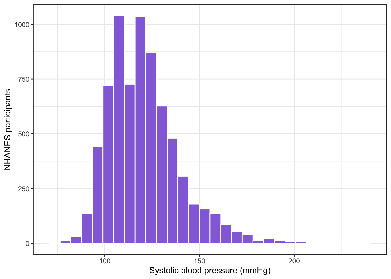
R Code 6.6 : Histogram of systolic blood pressure (NHANES 2015-2016)
Code
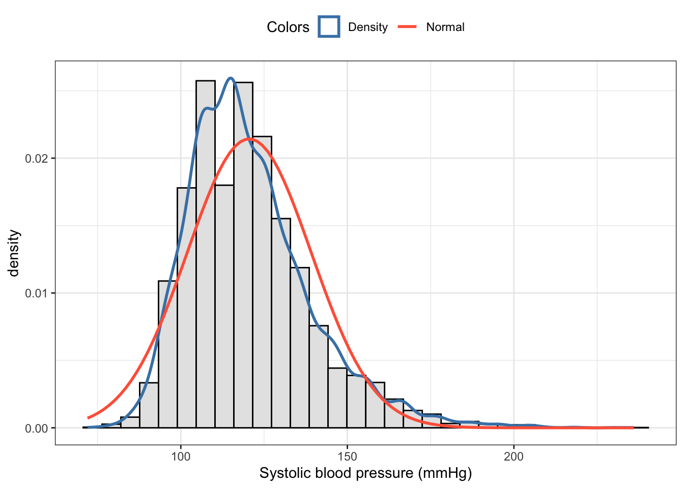
## load bpx_2016 #######bpx_2016<-base::readRDS("data/chap06/bpx_2016.rds")## graph systolic blood pressure variable BPXSY1 (Figure 6.1)sys_histo<-bpx_2016|>ggplot2::ggplot(ggplot2::aes(x =BPXSY1))+ggplot2::geom_histogram( fill ="mediumpurple", color ="white", bins =30, na.rm =TRUE)+ggplot2::theme_bw()+ggplot2::labs( x ="Systolic blood pressure (mmHg)", y ="NHANES participants")sys_histo
Histogram of systolic blood pressure (NHANES 2015-2016)
This is the replication of the book’s Figure 6.1.
The graph is not exactly normally distributed; it has a little right skew. The quantile values (0% 25% 50% 75% 100%) are 72, 108, 118, 130, 236. The middle 50% lies in the range between 108 and 130 mmHG. You can’t see the highest values because their frequencies are too small.
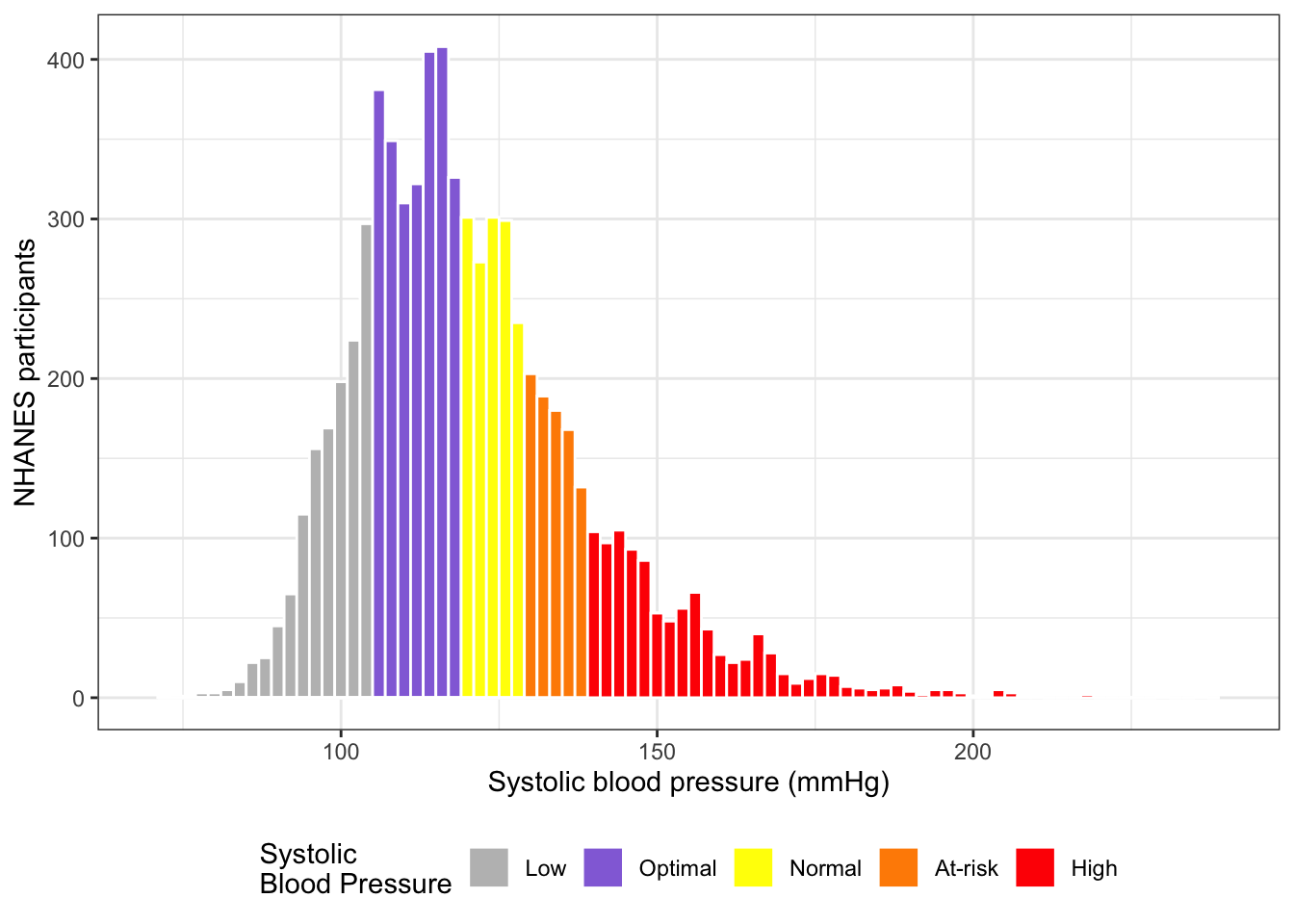
R Code 6.7 : Histogram of systolic blood pressure with risk factors (NHANES 2015-2016)
Code
## graph systolic blood pressure with risk factors (Figure 6.2)sys_histo2<-bpx_2016|>ggplot2::ggplot(ggplot2::aes( x =BPXSY1, fill =BPXSY1>120))+ggplot2::geom_histogram( color ="white", bins =30, na.rm =TRUE)+ggplot2::theme_bw()+ggplot2::labs( x ="Systolic blood pressure (mmHg)", y ="NHANES participants")+ggplot2::scale_fill_manual( values =c("mediumpurple", "grey"), labels =c("Normal range","at-risk or high"), name ="Systolic\nBlood Pressure")sys_histo2
Histogram of systolic blood pressure with risk factors (NHANES 2015-2016)
This is the replication of the book’s Figure 6.2.
R Code 6.8 : Blood pressure histogram with several colors according to their medical conditions
Code
## graph systolic blood pressure differentiatedsys_histo3<-bpx_2016|>dplyr::select(BPXSY1)|>dplyr::mutate(sys =dplyr::case_when(BPXSY1<105~"0",BPXSY1>=105&BPXSY1<120~"1",BPXSY1>=120&BPXSY1<130~"2",BPXSY1>=130&BPXSY1<140~"3",BPXSY1>=140~"4"))|>ggplot2::ggplot(ggplot2::aes(x =BPXSY1, fill =sys))+ggplot2::geom_histogram( color ="white", binwidth =2, na.rm =TRUE)+ggplot2::theme_bw()+ggplot2::theme(legend.position ="bottom")+ggplot2::labs( x ="Systolic blood pressure (mmHg)", y ="NHANES participants")+ggplot2::scale_fill_manual( values =c("0"="grey", "1"="mediumpurple", "2"="yellow", "3"="darkorange", "4"="red"), labels =c("Low","Optimal","Normal","At-risk","High"), name ="Systolic\nBlood Pressure")+ggplot2::xlim(70, 240)sys_histo3
Here I have experimented to colorize the histogram with different colors. I took as borders the medical condition for isolated blood pressure measures:
Low: < 105
Optimal: >= 105 & < 120
Normal: >= 120 & < 130
At Risk: >= 130 & < 140
High: >= 140
In this case I can’t use the color directly as fill variable into the ggplots::aes() function. Besides I learned two other solve two other issues:
The sequence of colors are aligned to the values alphabetically. Therefore I had to take characters that are sorted in the correct order. I took c(“0”, “1”, “2”, “3”, “4”) but c(“a”, “b”, “c”, “d” ,“e”) would have worked too.
Wider bins brought the problem that the color has changed in the middle of the bar length. I did not know how to solve this issue generally, for instance with providing breaks or to provide borders conforming to the medical status. Only binwidth of 1 and 2 worked, 3 already showed the problem. Other people had the same problem, see for instance the section “Example 2: Draw Histogram with Different Colors Using ggplot2 Package” in Draw Histogram with Different Colors in R (2 Examples)(Schork, n.d.).
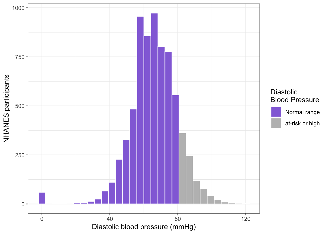
R Code 6.9 : Histogram of diastolic blood pressure with risk factors (NHANES 2015-2016)
Code
## graph systolic blood pressure with risk factors (Figure 6.3)dia_histo<-bpx_2016|>ggplot2::ggplot(ggplot2::aes( x =BPXDI1, fill =BPXDI1>80))+ggplot2::geom_histogram( color ="white", bins =30, na.rm =TRUE)+ggplot2::theme_bw()+ggplot2::labs( x ="Diastolic blood pressure (mmHg)", y ="NHANES participants")+ggplot2::scale_fill_manual( values =c("mediumpurple", "grey"), labels =c("Normal range","at-risk or high"), name ="Diastolic\nBlood Pressure")dia_histo
Histogram of diastolic blood pressure with risk factors (NHANES 2015-2016)
This is the replication of the book’s Figure 6.3.
R Code 6.10 : Mean and standard deviation of systolic blood pressure in the NHANES data sample (2015-2016)
Code
bpx_stats<-bpx_2016|>tidyr::drop_na(BPXSY1)|>dplyr::summarize( mean =base::mean(BPXSY1), sd =stats::sd(BPXSY1), n =dplyr::n())bpx_stats
#>       mean       sd    n
#> 1 120.5394 18.61692 7145
6.5 Achievement 2: One-Sample t-test
6.5.1 Introduction
We have a mean of the systolic blood pressure a little bit above 120.54 mmHG. This is almost exactly the upper cutoff value of 120 mmHG for the “normal range” of blood pressure. Is this only valid for the sample of also for the whole population? Have about half of the US people high systolic blood pressure, e.g. more than 120mmHG? The question can be answered with a one-sample t-test. The one sample t-test compares a sample mean to a hypothesized or population mean.
There are three different t-tests
One-sample t-test: compares a mean to a population or hypothesized value
Independent-samples t-test: compares the means of two unrelated groups
Dependent-samples t-test: compares the means of two related groups
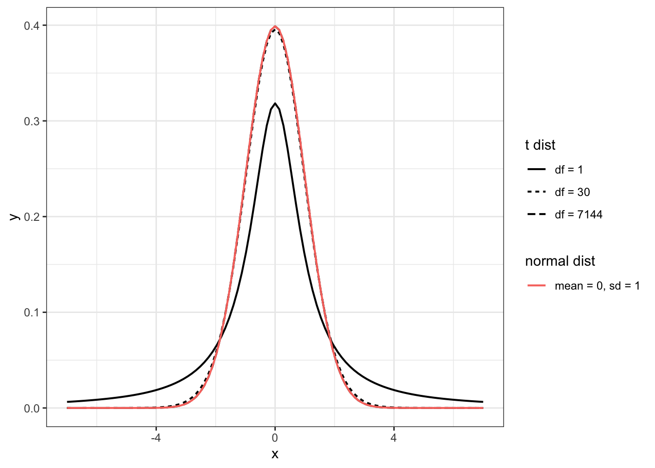
The t-distribution has a bell shape like the normal distribution. But unlike the normal distribution its variance is not known but approximated with its only parameter degrees of freedom (df). df is calculated by the number of observations minus one (\(n-1\)). With higher degrees of freedom the t-distribution will get closer to the normal distribution. Often the number 30 is recommended as the cutting point where t-distribution and normal distribution are equivalent.
The Null relates most of the times to a situation where no change occurs. In this case that there is no difference in the means of the systolic blood pressure. This is different to the assumption that the mean difference is not higher than 120 mmHG!
In the one-sample t-test we are comparing sample mean with population mean. In this case the NHANES sample from the 2015-2016 data with the population mean of the US population.
Wording for H0 and HA
H0: There is no difference in the mean systolic blood pressure in the US population and the cutoff for normal blood pressure of 120 mmHG in the NHANES 2015-2016 data set.
HA: There is a difference in the mean systolic blood pressure in the US population and the cutoff for normal blood pressure of 120 mmHG in the NHANES 2015-2016 data set.
6.5.3 NHST Step 2
Compute the test statistic. The one-sample t-test uses the t-statistic (sort of like a z-statistic)
Formula 6.1 : t-test formula
\[
t = \frac{m_{x} - \mu_{x}}{\frac{s_x}{\sqrt{n_{x}}}}
\tag{6.1}\]
\(m_{x}\) represents the mean of the variable x, the variable to be tested,
\(\mu_{x}\) is the population mean or hypothesized value of the variable,
\(s_{x}\) is the sample standard deviation of x, and
z shows how many sample standard deviations some value is away from the mean.
t shows how many standard errors (i.e., population standard deviations) some value is away from the mean.
\[
t = \frac{120.5394 - 120}{\frac{18.61692}{\sqrt{7145}}} = 2.45
\]
R Code 6.11 : t-statistic of systolic blood pressure aof NHANES sample with hypothesized population mean
Code
(t_test_systolic<-stats::t.test(bpx_2016$BPXSY1, alternative ="two.sided", mu =120))
#>
#>  One Sample t-test
#>
#> data:  bpx_2016$BPXSY1
#> t = 2.4491, df = 7144, p-value = 0.01435
#> alternative hypothesis: true mean is not equal to 120
#> 95 percent confidence interval:
#>  120.1077 120.9711
#> sample estimates:
#> mean of x
#>  120.5394
Code
## for later use #########t_sys=t_test_systolic[["statistic"]][["t"]]df_sys=t_test_systolic[["parameter"]][["df"]]null_sys=t_test_systolic[["null.value"]][["mean"]]estimate_sys=t_test_systolic[["estimate"]][["mean of x"]]p_value_sys=t_test_systolic[["p.value"]]se_sys=t_test_systolic[["stderr"]]
I have stored the result of the t-test into variables for later use.
Assessment 6.1 : Explications of the t-test output
1. Line: Data (variable) used. 2. Line: - t: value of the t-test statistic. - df: degrees of freedom, with t-statistic = subtracting 1 from sample size = \(n - 1\). - p-value: The probability of the sample coming from a population where the null hypothesis is true. 3. Line: wording of the alternative hypothesis. 4. Line: Chosen confidence interval. 5. Line: The lower and upper boundary of the confidence interval. 6. Line: Sample estimates that has to be compared to the value of the null hypothesis.
6.5.4 NHST Step 3
Review and interpret the test statistics: Calculate the probability that your test statistic is at least as big as it is if there is no relationship (i.e., the null is true).
The following examples replicates Figure 6.4, 6.5 and 6.6. I will break down the final code into several steps following the nice article [Visualizing Sampling Distributions: Learn how to add areas under the curve in sampling distributions]https://ggplot2tutor.com/tutorials/sampling_distributions (Burkhart 2021).
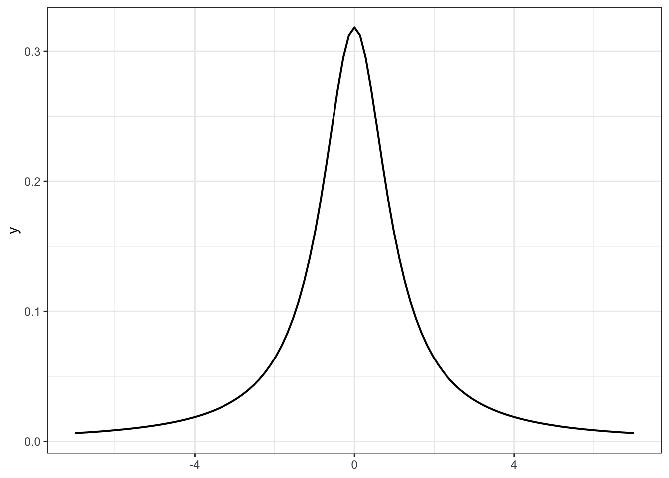
Example 6.4 : Probability distribution of t-test statistic
R Code 6.12 : Student t distributions with 1 degree of freedom (df)
Code
ggplot2::ggplot()+ggplot2::xlim(-7, 7)+## or as an alternative# ggplot2::ggplot(tibble::tibble(x = c(-7, 7)), # ggplot2::aes(x)) +ggplot2::stat_function( fun =stats::dt, args =list(df =1), geom ="line", linewidth =0.7)+ggplot2::theme_bw()
Graph 6.1: Student t distributions with 1 degree of freedom (df)
Procedure 6.1 : Plotting a distribution with {ggplot2}
As there is no data (just the formula for the function) we need to specify the x-limits.
ggplot2::stat_function draws the function. We can specify the function extra or create an anonymous function or — as I have done here — use a function from an R package. Note that there is no parenthesis behind the function name.
R Code 6.13 : Student t distributions with 1 and 7144 degree of freedom (df) and normal distribution compared
Add for each legend a corresponding scale with name and labels.
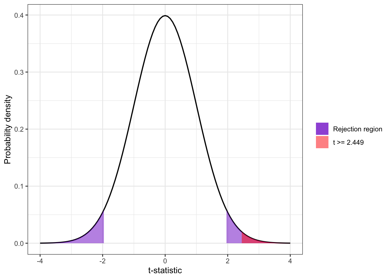
R Code 6.14 : t-distribution (df = 7,144) shaded for values of 2.4491 or higher (replicating Figure 6.5)
Code
ggplot2::ggplot()+ggplot2::xlim(-4, 4)+ggplot2::stat_function( fun =stats::dt, args =list(df =df_sys), geom ="line", linewidth =0.7)+ggplot2::stat_function( fun =stats::dt, args =list(df =df_sys), geom ="area", xlim =c(t_sys, 4),ggplot2::aes(fill =paste("t >=", round(t_sys, 3))))+ggplot2::theme_bw()+ggplot2::scale_fill_manual( name ="", values ="steelblue")
Graph 6.3: t-distribution (df = 7,144) shaded for values of 2.4491 or higher (replicating Figure 6.5)
The plot shows that the t-value of 2.499 is very unlikely if the null hypotheses were true, e.g. if the sample comes from a population with a systolic blodd pressure mean of 240.
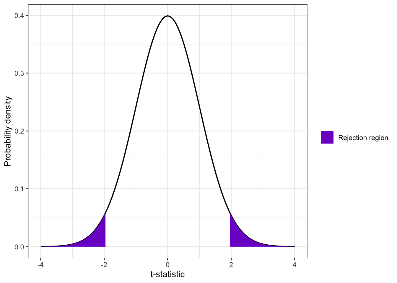
R Code 6.15 : t-distribution (df = 7,144) with 2.5% shaded in each tail of the distribution (replicating Figure 6.6)
Code
ggplot2::ggplot()+ggplot2::xlim(-4, 4)+ggplot2::stat_function( fun =stats::dt, args =list(df =df_sys), geom ="line", linewidth =0.7)+ggplot2::stat_function( fun =stats::dt, args =list(df =df_sys), geom ="area", xlim =c(1.96, 4),ggplot2::aes(fill =paste("Rejection region")))+ggplot2::stat_function( fun =stats::dt, args =list(df =df_sys), geom ="area", xlim =c(-4, -1.96),ggplot2::aes(fill =paste("Rejection region")))+ggplot2::theme_bw()+ggplot2::scale_fill_manual( name ="", values ="purple3")+ggplot2::labs( x ="t-statistic", y ="Probability density")
Graph 6.4: t-distribution (df = 7,144) with 2.5% shaded in each tail of the distribution (replicating Figure 6.6)
The plot shows the rejection regions for the probability of 95%.
R Code 6.16 : t-distribution (df = 7,144) with 2.5% shaded in each tail of the distribution (replicating Figure 6.6)
Code
ggplot2::ggplot()+ggplot2::xlim(-4, 4)+ggplot2::stat_function( fun =stats::dt, args =list(df =df_sys), geom ="line", linewidth =0.7)+ggplot2::stat_function( fun =stats::dt, args =list(df =df_sys), geom ="area", xlim =c(1.96, 4), alpha =0.5,ggplot2::aes(fill =paste("Rejection region"),))+ggplot2::stat_function( fun =stats::dt, args =list(df =df_sys), geom ="area", xlim =c(-4, -1.96), alpha =0.5,ggplot2::aes(fill =paste("Rejection region"),),)+ggplot2::stat_function( fun =stats::dt, args =list(df =df_sys), geom ="area", xlim =c(t_sys, 4), alpha =0.5,ggplot2::aes(fill =paste("t >=", round(t_sys, 3))))+ggplot2::theme_bw()+ggplot2::scale_fill_manual( name ="", values =c("purple3", "red"))+ggplot2::labs( x ="t-statistic", y ="Probability density")
Graph 6.5: t-distribution (df = 7,144) with 2.5% shaded in each tail of the distribution (replicating Figure 6.6)
The plot shows that the t-value is in the rejection area, e.g., the null has to be rejected.
6.5.5 NHST Step 4
Conclude and write the report.
Even though the difference between the mean systolic blood pressure of 120.54 and the hypothesized value of 120 is small, it is statistically significant. The probability of this sample that it comes from a population where the mean systolic blood pressure is actually 120 is just 1.4%. This sample is likely to be from a population with a higher mean blood pressure.
Report
The mean systolic blood pressure in a sample of 7145 people was 120.54 (sd = 18.62). A one-sample t-test found this mean to be statistically significantly different from the hypothesized mean of 120 [t(7144) = 2.449; p = 0.014]. The sample likely came from a population with a mean systolic blood pressure not equal to 120.
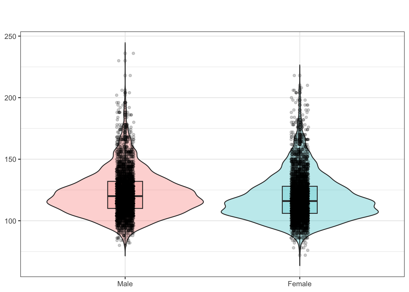
6.6 Achievement 3: Independent-samples t-test
Instead of comparing one mean to a hypothesized or population mean, the independent-samples t-test compares the means of two groups to each other.
We could for instance be interested to see if the blood pressure for persons of different sex are the same. Or the question statistically formulated: Do males and females in the sample come from a population where males and females have the same mean systolic blood pressure?
I am not going into the details of achievement 3 because there is no much difference between the procedure for the one-sample t-test and the independent-samples t-test. Essentially there are only two differences:
6.6.1 Formula
Formula 6.2 : Independent-samples t-test formula
\[
t = \frac{m_{1} - m_{2}}{\sqrt{\frac{s_1^2}{n_{1}} + \frac{s_2^2}{n_{2}}}}
\tag{6.2}\]
\(m_{1}\) represents the mean of one group,
\(m_{2}\) represents the mean of another group,
\(s_{1}^2\) is the variance of the first group,
\(s_{2}^2\) is the variance of the second group,
\(n_{1}\) is the size of the first group,
\(n_{2}\) is the size of the second group.
6.6.2 Computing
R Code 6.17 : Independent-samples t-test for systolic blood pressure of males and females
#> # A tibble: 2 × 4
#>   sex    mean_systolic var_systolic sample_size
#>   <fct>          <dbl>        <dbl>       <int>
#> 1 Male            122.         329.        3498
#> 2 Female          119.         358.        3647
#>
#>  Welch Two Sample t-test
#>
#> data:  bp_clean$systolic by bp_clean$sex
#> t = 7.3135, df = 7143, p-value = 2.886e-13
#> alternative hypothesis: true difference in means between group Male and group Female is not equal to 0
#> 95 percent confidence interval:
#>  2.347882 4.067432
#> sample estimates:
#>   mean in group Male mean in group Female
#>             122.1767             118.9690
Listing / Output 6.2: Independent-samples t-test for systolic blood pressure of males and females
It is important to note that category variables like sex do not work with the default x, y version of the t-test. Therefore we have to apply the method with class formula.
In R formulae a single variable on the left-hand side is followed by the tilde sign ~ and one ore more objects that predict or explain the left-hand side.
In a lot of statistical tests, the object on the left-hand side of the formula is the outcome or dependent variable while the object(s) on the right-hand side of the formula are the predictors or independent variables. (SwR)
It is commonly used to generate design matrices for modeling function (e.g. lm) (Kuhn 2017).
In our case, systolic blood pressure is the outcome being explained by the predictor of sex.
In R the default t-test for independent samples is the Welch’s t-test and not the student t-test.
Welch’s t-test is slightly different from the original formula for t, which used pooled variance in the denominator. Pooled variance assumes that the variances in the two groups are equal and combines them. (SwR)
There is an scientific article explaining why Welch’s t-test should be used in any case, even if the assumption of homogeneity of variance is met:
We show that the Welch’s t-test provides a better control of Type 1 error rates when the assumption of homogeneity of variance is not met, and it loses little robustness compared to Student’s t-test when the assumptions are met. We argue that Welch’s t-test should be used as a default strategy. (Delacre, Lakens, and Leys 2017; see also: Delacre, Lakens, and Leys 2022)
Just to conclude this abbreviated section I quote the final summary reporting the independent t-test results.
Report
There was a statistically significant difference [t(7143) = 7.31; p < .05] in mean systolic blood pressure between males (m = 122.18) and females (m = 118.97) in the sample. The sample was taken from the U.S. population, indicating that males in the United States likely have a different mean systolic blood pressure than females in the United States. The difference between male and female mean systolic blood pressure was 3.21 in the sample; in the population this sample came from, the difference between male and female mean blood pressure was likely to be between 2.35 and 4.07 (d = 3.21; 95% CI: 2.35–4.07). (SwR)
6.7 Achievement 4: Dependent-samples t-test
Again: I am not going to summarize this section because it resembles achievement 2 (one-sample t-test) and achievement 3 (independent.samples t-test).
6.7.1 Formula
Formula 6.3 : Independent-samples t-test formula
\[
t = \frac{m_{d} - 0}{\sqrt{\frac{s_d}{n_{d}}}}
\tag{6.3}\]
\(m_{d}\) represents the mean of differences between to measures,
\(s_{d}^2\) is the variance of the mean differences between to measures,
\(n_{d}\) is the sample size,
\(0\) subtracting represents the null hypothesis; zero is the mean difference if the two measures were exactly the same.
6.7.2 Computing
General advice before starting a test statistics
Always look at some visuals and descriptive statistics before you are starting the test procedure and following the NHST procedure as outlined in Procedure 5.2.
This shows that the difference of the mean between two measures is very small (0.55 mmHG). But it turned out that this value is highly statistically significant. But from a clinical point of view it is irrelevant!
Statistically significant != meaningful!
All our three t-tests result in small but statistically significant values. This is an important reminder that statistically significant p-values are not necessarily of relevance.
By the way: The reason for our small but statistically significant values are very large samples.
The computation in R is the same as in Listing / Output 6.2. Again apply the formula version of Welch’s t-test with the only difference to add the argument paired = TRUE.
6.8 Achievement 5: Effect size
6.8.1 Introduction
We haven seen that even the very small difference of 0.54 mmHG systolic blood pressure is with a large sample size statistically significant. But this small difference is clinically not relevant. To judge the importance of some statistically significant results we need effect sizes as another criteria.
The proportion of people that believe that effect sizes are even more important than p-values is rising. P-values only report whether a difference or relationship from a sample is likely to be true in the population, while effect sizes provide information about the strength or size of a difference or relationship.
In Chapter 5 we discussed for the Chi-squared test as effect sizes
For t-test the appropriate effect size measure is Cohen’s d.
Resource 6.2 Delving into effect size assessment
Derived from the importance of effect size parameter I need to know more how to use and interpret different kind of effect sizes. What follows are some resources
Thee is another package {effsize} that I have not used. I had problems to use it, because it has no argument for \(\mu\) but it also has not many downloads.
The packages {effectsize} and {rstatix} are important as they have many other computation for effect size parameters.
Table 6.1: Download average numbers of packages with Cohen’s d functions
The effect size is very small, it is not even close the starting value for “small effect size”.
Report
The mean systolic blood pressure in a sample of 7,145 people was 120.54 (sd = 18.62). A one-sample t-test found this mean to be statistically significantly different from the hypothesized mean of 120 [t(7144) = 2.45; p = 0.014]. The sample likely came from a population with a mean systolic blood pressure not equal to 120. While the sample mean was statistically significantly different from 120, is has a very small effect size (Cohen’s d = .03).
R Code 6.19 : Compute Cohen’s d with for one-sample t-tests {lsr}
R Code 6.20 : Compute Cohen’s d for one-sample t-tests with {effectsize}
Code
effectsize::cohens_d( x =bp_clean$systolic, mu =120)
#> Warning: Missing values detected. NAs dropped.
#> Cohen's d |       95% CI
#> ------------------------
#> 0.03      | [0.01, 0.05]
#>
#> - Deviation from a difference of 120.
The {effectsize} packages discusses two alternatives for Cohen’s d:
Hedges’ g provides a correction for small-sample bias (using the exact method) to Cohen’s d. For sample sizes > 20, the results for both statistics are roughly equivalent.
Glass’s delta is appropriate when the standard deviations are significantly different between the populations, as it uses only the second group’s standard deviation.
R Code 6.21 : Compute Cohen’s d for one-sample t-tests with {rstatix}
Code
rstatix::cohens_d( data =bp_clean, formula =systolic~1, mu =120)
#> # A tibble: 2 × 3
#>   sex    mean_sys_sex var_sys_sex
#>   <fct>         <dbl>       <dbl>
#> 1 Male           122.        329.
#> 2 Female         119.        358.
#> [1] 0.1730045
The effect size is very small.
R Code 6.23 : Compute Cohen’s d of independent samples with {lsr}
Code
lsr::cohensD( x =systolic~sex, data =bp_clean, method ="unequal")
#> [1] 0.1730045
Instead of a vector variable we are using the formula interface.
Because we are using the Welch’s t-test we change the default method “pooled”, to “unequal”, e.g., we are not assuming equal variances.
R Code 6.24 : Compute Cohen’s d for independent-samples t-tests with {effectsize}
Code
effectsize::cohens_d( x =bp_clean$systolic, y =bp_clean$sex, pooled_sd =FALSE, paired =FALSE)
#> Warning: Missing values detected. NAs dropped.
#> Cohen's d |       95% CI
#> ------------------------
#> 0.17      | [0.13, 0.22]
#>
#> - Estimated using un-pooled SD.
The {effectsize} packages discusses two alternatives for Cohen’s d:
Hedges’ g provides a correction for small-sample bias (using the exact method) to Cohen’s d. For sample sizes > 20, the results for both statistics are roughly equivalent.
Glass’s delta is appropriate when the standard deviations are significantly different between the populations, as it uses only the second group’s standard deviation.
R Code 6.25 : Compute Cohen’s d for independent-samples t-tests with {rstatix}
Code
rstatix::cohens_d( data =bp_clean, formula =systolic~sex)
R Code 6.27 : Compute Cohen’s d of dependent samples with {lsr}
Code
lsr::cohensD( x =bp_clean$systolic, y =bp_clean$systolic2, method ="paired")
#> [1] 0.1112676
Instead of the default method (“pooled”) we need “paired” as method for the dependent-samples t-test.
R Code 6.28 : Compute Cohen’s d for dependent-samples t-tests with {effectsize}
Code
effectsize::cohens_d( x =bp_clean$systolic, y =bp_clean$systolic2, paired =TRUE)
#> Warning: Missing values detected. NAs dropped.
#> For paired samples, 'repeated_measures_d()' provides more options.
#> Cohen's d |       95% CI
#> ------------------------
#> 0.11      | [0.09, 0.13]
The {effectsize} packages discusses two alternatives for Cohen’s d:
Hedges’ g provides a correction for small-sample bias (using the exact method) to Cohen’s d. For sample sizes > 20, the results for both statistics are roughly equivalent.
Glass’s delta is appropriate when the standard deviations are significantly different between the populations, as it uses only the second group’s standard deviation.
R Code 6.29 : Compute Cohen’s d for dependent-samples t-tests with {rstatix}
In order to get a working cohen’s d computation with {rstatix} I had to apply tidyr::pivot_longer().
6.9 Achievement 6: t-test assumptions
6.9.1 Introduction
In this section I am not following the sequence of the book. I start with an overview and will separate - checking visually the normality assumption - testing with different approaches the normality assumption
Bullet List
One-sample t-test assumptions
Continuous variable
Independent observations
Normal distribution
Independent-samples t-test assumptions
Continuous variable and two independent groups
Independent observations
Normal distribution in each group
Equal variances for each group
Dependent-samples t-test assumptions
Continuous variable and two dependent groups
Independent observations
Normal distribution of differences
Bullet List 6.1: Assumptions for the different t-tests
6.9.2 Checking normality assumption visually
6.9.2.1 One-sample t-test
Example 6.7 : One-sample t-test: Checking the normality assumption visually
Graph 6.6: Distribution of systolic blood pressure in mmHg for 20152016 NHANES participants (30 bins)
The data appear right-skewed, e.g. the right tail is longer than the left tail. There is also the assumption that the distribution is bimodal, e.g., has two modes.
The best way to check if this assumption is correct is to change the number of bins.
R Code 6.31 : Checking normality visually (60 bins)
Graph 6.7: Distribution of systolic blood pressure in mmHg for 20152016 NHANES participants (60 bins)
Another graph — this time with 60 bins — shows that we have a unimodal distribution.
R Code 6.32 : Checking normality visually with a Q-Q plot
Code
bp_clean2|>ggplot2::ggplot(ggplot2::aes(sample =systolic))+ggplot2::stat_qq(ggplot2::aes(color ="NHANES participant"))+ggplot2::stat_qq_line(ggplot2::aes(linetype ="Normally distributed"), linewidth =1)+ggplot2::labs( x ="Theoretical normal distribution", y ="Observes systolic blood pressure (mmHG)")+ggplot2::scale_color_manual( name ="", values =("NHANES participant"="purple3"))+ggplot2::scale_linetype_manual( name ="", values =("Normally distributed"="solid"))
Graph 6.8: Distribution of systolic blood pressure in mmHg for 2015-2016 NHANES participants
(This is the replication of book Figure 6.12, that has no accompanying code.)
This q-q-plot shows clearly that we have failed the assumption of a normal distribution. But often the visible check is not so obvious. Then we would need a statistical test to check for normality.
6.9.2.2 Independent-samples t-test
Normality has to be checked for each group for the independent-samples t-test (and dependent-samples t-test).
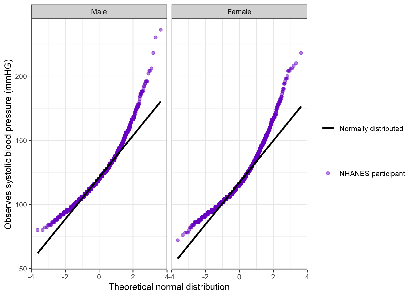
Example 6.8 : Independent-samples t-test: Checking the normality assumption visually
bp_clean<-base::readRDS("data/chap06/bp_clean.rds")bp_clean|>ggplot2::ggplot(ggplot2::aes(x =systolic))+ggplot2::geom_histogram( fill ="purple3", col ="white", na.rm =TRUE, bins =30)+ggplot2::facet_grid( cols =ggplot2::vars(sex))+ggplot2::labs( x ="Systolic blood pressure (mmHg)", y ="NHANES participants")
Graph 6.9: Distribution of systolic blood pressurein mmHg for 20152016 NHANES participants by sex
Both histograms look right-skewed.
R Code 6.34 : Checking normality with Q-Q plot
Code
bp_clean|>tidyr::drop_na(systolic)|>ggplot2::ggplot(ggplot2::aes(sample =systolic))+ggplot2::stat_qq(ggplot2::aes(color ="NHANES participant"), alpha =0.5)+ggplot2::stat_qq_line(ggplot2::aes(linetype ="Normally distributed"), linewidth =1)+ggplot2::facet_grid( cols =ggplot2::vars(sex))+ggplot2::labs( x ="Theoretical normal distribution", y ="Observes systolic blood pressure (mmHG)")+ggplot2::scale_color_manual( name ="", values =("NHANES participant"="purple3"))+ggplot2::scale_linetype_manual( name ="", values =("Normally distributed"="solid"))
Graph 6.10: Checking normality of systolic blood pressure in mmHg for 20152016 NHANES participants by sex with Q-Q plots
Harris uses in the book a more complicated code passage to build the line for the normal distribution. Instead using the function ggplot2::stat_qq_line() she calculates intercept and slopes and applies the ggplot2::abline() function.
The q-q plot shows that both blood pressures (males and females) are not normally distributed.
6.9.2.3 Dependent samples t-test
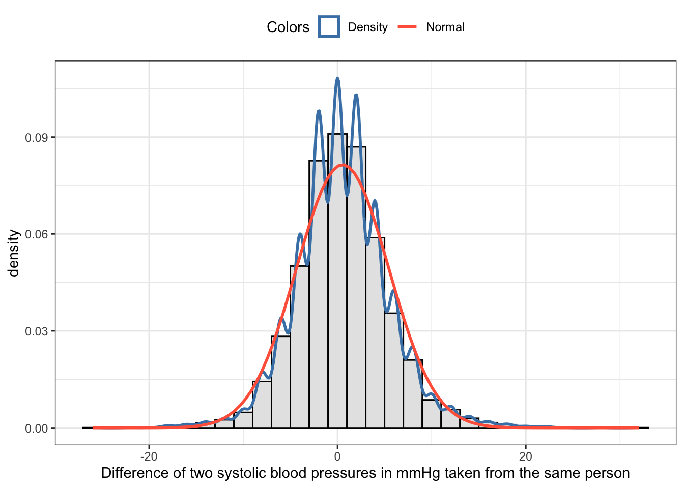
Here we are going to check the distribution of the difference between the first (systolic) and second blood pressure measure (systolic2).
Example 6.9 : Dependent-samples t-test: Checking the normality assumption visually
R Code 6.35 : Checking the normality assumption visually with a histogram and an overlaid normal distribution
Code
bp_clean<-base::readRDS("data/chap06/bp_clean.rds")bp_clean3<-bp_clean|>tidyr::drop_na(diff_syst)my_hist_dnorm( df =bp_clean3, v =bp_clean3$diff_syst, n_bins =30, x_label ="Difference of two systolic blood pressures in mmHg taken from the same person")
Graph 6.11: Checking the normality assumption visually of a dependent group distribution with a histogram and an overlaid normal distribution
The histogram looks like a normal distribution. But let’s verify this rsult with a q-q plot.
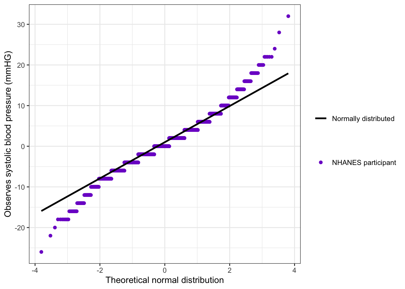
R Code 6.36 : Checking the normality assumption visually with a quantile-quantile plot
Code
bp_clean3|>ggplot2::ggplot(ggplot2::aes(sample =diff_syst))+ggplot2::stat_qq(ggplot2::aes(color ="NHANES participant"))+ggplot2::stat_qq_line(ggplot2::aes(linetype ="Normally distributed"), linewidth =1)+ggplot2::labs( x ="Theoretical normal distribution", y ="Observes systolic blood pressure (mmHG)")+ggplot2::scale_color_manual( name ="", values =("NHANES participant"="purple3"))+ggplot2::scale_linetype_manual( name ="", values =("Normally distributed"="solid"))
Graph 6.12: Checking the normality assumption visually of a dependent group distribution with a quantile-qunatile plot
Bad news! This is a disappointing result: Th Q-Q plot shows that we do not have normal distribution. It just looked like one as the lower and higher values cancel each out.
6.9.2.4 Summary of the visual inspections
For all t-tests we applied in this chapter we got the clear result that they all failed the normality assumption.
But often the visual inspection is not conclusive. Therefore it is important also to apply statistical tests.
6.9.3 Checking normality assumption with statistical tests
6.9.3.1 Skewness
Different statistical checks for normality for different situations
Different statistical checks of normality are useful in different situations.
The mean of a variable is sensitive to skew, so checking for skewness (Section 2.6.2) is important when a statistical test relies on means (like t-tests).
When the focus of a statistical test is on variance, it is a good idea to examine kurtosis (Section 2.6.4) because variance is sensitive to problems with kurtosis (e.g., a platykurtic or leptokurtic distribution)
Resource 6.4 Packages with tests for skewness
After another research I will — in addition to Section 2.6.2 — propose other packages with tests for skewness. A comparison shows that these tests are much more popular given their download figures as the two packages (Section A.80 and Section A.85) I have already reviewed. All of the mentioned packages have functions for tests for kurtosis as well.
{datavizard}: Easy Data Wrangling and Statistical Transformations
{e1071}: Misc Functions of the Department of Statistics, Probability Theory Group (Formerly: E1071), TU Wien
{moments}: Moments, Cumulants, Skewness, Kurtosis and Related Tests
{psych}: Procedures for Psychological, Psychometric, and Personality Research
Table 6.2: Download average numbers of packages with skewness functions
#> Warning in semTools::skew(bp_clean$systolic): Missing observations are removed
#> from a vector.
#>   skew (g1)          se           z           p
#>  1.07037232  0.02897841 36.93689298  0.00000000
Comparing the z-value in Table 2.10 we see that our value is 5 times higher than 7, meaning our distribution is highly right skewed. With a p-value < 0.001 we have to reject the null (that we have a normal distribution).
R Code 6.38 : Compute skewness of systolic blood pressure with {e1071}
Code
e1071::skewness( x =bp_clean$systolic, na.rm =TRUE, type =2)
#> [1] 1.070372
There are three slightly different types of skewness computation with {e1071}.
Type 1: Older textbooks (‘classic’)
Type 2: SAS and SPSS
Type 3: MINITAB and BMDP (default value)
If we compare with the skewness computation of {semTools} we see that SAS/SPSSS calculation is used with type 2 in {e1071}.
We can’t assess the skewness with Table 2.10, because {e1071} does not calculate the z- and p-value. We therefore add another assessment criteria for skewness:
Assessment 6.3 : Magnitude of skewness
If the skewness value is close to 0 (between -0.5 and 0.5), the distribution is approximately symmetric.
If the skewness value is significantly negative (below -1), it suggests strong left skewness.
If the skewness value is significantly positive (above 1), it suggests strong right skewness. (GeeksforGeeks) (parmarraman44 2023).
A value above 1.0 suggests a strong right skewness.
R Code 6.39 : Compute skewness of systolic blood pressure with {moments}
Code
moments::skewness( x =bp_clean$systolic, na.rm =TRUE)
#> [1] 1.070148
This slightly different value would be the result in {e1071} with type = 1 (older textbooks).
R Code 6.40 : Compute skewness of systolic blood pressure with {datawizard}
Code
(sys_skew_datawizard<-datawizard::skewness( x =bp_clean$systolic, remove.na =TRUE, type =2# default))base::summary(sys_skew_datawizard, test =TRUE)
#> Skewness |    SE
#> ----------------
#>    1.070 | 0.029
#> Skewness |    SE |      z | p
#> -----------------------------
#>    1.070 | 0.029 | 36.952 | 0
There are two versions with {datawizard}. One with just the skewness and standard error, another one — similar as with {semTools} — with skewness, standard error, z-value and p-value.
R Code 6.41 : Compute skewness of systolic blood pressure with {psych}
Code
psych::skew( x =bp_clean$systolic, type =2)(sys_mardia_psych<-psych::mardia(bp_clean$systolic))
#> [1] 1.070372
#> Call: psych::mardia(x = bp_clean$systolic)
#>
#> Mardia tests of multivariate skew and kurtosis
#> Use describe(x) the to get univariate tests
#> n.obs = 7145   num.vars =  1
#> b1p =  1.14   skew =  1363.19  with probability  <=  2.1e-298
#>  small sample skew =  1364.33  with probability <=  1.2e-298
#> b2p =  4.99   kurtosis =  34.33  with probability <=  0
There are two different approaches with {psych}:
A simple calculation of the skewness, very similar to the computation of {e1071}
A much more detailed result with the option to plot a q-q- plot to test normality.
R Code 6.42 : Statistical test of normality for systolic blood pressure by sex
#>    skew (g1)           se            z            p
#> 2.351789e-01 2.906805e-02 8.090632e+00 6.661338e-16
The skewness value is much lower but still over the limit of 7 for our sample size. So the null has to be rejected (p-value < 0001).
6.9.3.2 Different omnibus tests
Besides of testing skewness there are also other statistical tests available. I have researched the following omnibus tests:
Shapiro-Wilk: This is the book’s recommendation. The test is also called Shapiro-Francia and is a built-in test in R, available with stats::shapiro.test(). The test statistic of the Shapiro-Francia test is simply the squared correlation between the ordered sample values and the (approximated) expected ordered quantiles from the standard normal distribution. The Shapiro-Wilk test is known to perform well. But this test is very sensitive and can only be applied when the non-missing values are between 5 and 5000. With samples greater than 5,000 it will always result in statistically significant p-values. Therefore we can’t use it as we have a sample size of about 7000 non-missing values.
Anderson-Darling: The Anderson-Darling test is the recommended EDF test if there are more than seven values. It can be assessed via the {nortest} package, which is specialized for normality tests.
Cramer von Mises: It needs also more than 7 data values. Compared to the Anderson-Darling test (as a first choice) it gives less weight to the tails of the distribution.
Kolmogorov-Smirnov: Also called Liliefors test, needs at least 4 data values. The Lilliefors (Kolomorov-Smirnov) test is the most famous EDF omnibus test for normality. Compared to the Anderson-Darling test and the Cramer-von Mises test it is known to perform worse. Although the test statistic obtained from nortest::lillie.test() is the same as that obtained from stats::ks.test(), it is not correct to use the p-value from the latter for the composite hypothesis of normality (mean and variance unknown), since the distribution of the test statistic is different when the parameters are estimated.
Pearson: The Pearson chi-square test for normality is usually not recommended for testing the composite hypothesis of normality due to its inferior power properties compared to other tests.
6.9.3.3 Anderson-Darling test
Resource 6.5 Packages for the Anderson-Darling test
{cmstatr}: Statistical Methods for Composite Material Data (aerospace applications)
{DescTools}: Tools for Descriptive Statistics (Section A.15)
{kSamples}: K-Sample Rank Tests and their Combinations
I will use only the two most downloaded packages: {DescTools} because I have already installed it (see Section A.15) and {nortest} because it is a specialized package for test for normality and most articles refer to its usage.
#>
#>  Anderson-Darling normality test
#>
#> data:  bp_clean$systolic
#> A = 88.39, p-value < 2.2e-16
We’ve got a very tiny p-value so we have to reject the null hypothesis that the systolic blood pressure is normally distributed.
R Code 6.45 : One-sample t-test: Test of normality using the Anderson-Darling test with the {DescTools} package
Code
DescTools::AndersonDarlingTest( x =bp_clean2$systolic, null ="pnorm", mean =mean(bp_clean2$systolic), sd =sd(bp_clean2$systolic))
#>
#>  Anderson-Darling test of goodness-of-fit
#>  Null hypothesis: Normal distribution
#>  with parameters mean = 120.539, sd = 18.617
#>
#> data:  bp_clean2$systolic
#> An = 88.39, p-value = 8.397e-08
Again, we have to reject the Null.
The {DescTools} packages has the advantage that it is a general test of goodness-of-fit. Besides normality it could also be used to test other kind of distributions.
R Code 6.46 : Dependent-samples t-test: Test of normality using the Anderson-Darling test with {nortest} and {DescTools} package
Code
glue::glue("Computation with nortest package")nortest::ad.test(bp_clean$diff_syst)glue::glue(" ")glue::glue("###################################################")glue::glue("Computation with DescTools package")DescTools::AndersonDarlingTest( x =bp_clean3$diff_syst, null ="pnorm", mean =mean(bp_clean3$diff_syst), sd =sd(bp_clean3$diff_syst))
#> Computation with nortest package
#>
#>  Anderson-Darling normality test
#>
#> data:  bp_clean$diff_syst
#> A = 69.694, p-value < 2.2e-16
#>
#>
#> ###################################################
#> Computation with DescTools package
#>
#>  Anderson-Darling test of goodness-of-fit
#>  Null hypothesis: Normal distribution
#>  with parameters mean = 0.545, sd = 4.898
#>
#> data:  bp_clean3$diff_syst
#> An = 69.694, p-value = 8.45e-08
Both tests agree, even their p-values differ: We have to reject the Null.
6.9.4 Testing homogeneity of variances
6.9.4.1 Levene’s test
Homogeneity of variances is another assumption valid for the independent t-test. The data should be equally spread out in each group. Although we had used the Welch’s version of the t-test, which does not require homogeneity of variances, we will apply Levene’s test anyway. (An additional visual inspection via group-specific boxplots would helpful to gain a visual understanding of Levene’s test results.)
Resource 6.6 Packages for Levene’s test
{car}: Companion to Applied Regression {DescTools}: Tools for Descriptive Statistics {misty}: Miscellaneous Functions ‘T. Yanagida’ {rstatix}: Pipe-Friendly Framework for Basic Statistical Tests
Table 6.4: Download average numbers of packages with Levene’s test functions
#> # A tibble: 4 × 4
#>   package   average from       to
#>   <chr>       <dbl> <date>     <date>
#> 1 car         13044 2024-03-21 2024-03-27
#> 2 rstatix      5551 2024-03-21 2024-03-27
#> 3 DescTools    2099 2024-03-21 2024-03-27
#> 4 misty         804 2024-03-21 2024-03-27
The {car} packages is most of time used for Levene’s test. There is also a specific tidy() function in {broom} for the results of car::leveneTest().
Example 6.12 : Levene’s test with different packages
#> Levene's Test for Homogeneity of Variance (center = median)
#>         Df F value  Pr(>F)
#> group    1   3.552 0.05952 .
#>       7143
#> ---
#> Signif. codes:  0 '***' 0.001 '**' 0.01 '*' 0.05 '.' 0.1 ' ' 1
Report
The variances of systolic blood pressure for men and women are not statistically significantly different (p = .06), and the independent-samples t-test meets the assumption of homogeneity of variances.
R Code 6.48 : Testing for equal variances for systolic by sex with {DescTools}
Code
DescTools::LeveneTest( formula =systolic~sex, data =bp_clean)
#> Levene's Test for Homogeneity of Variance (center = median)
#>         Df F value  Pr(>F)
#> group    1   3.552 0.05952 .
#>       7143
#> ---
#> Signif. codes:  0 '***' 0.001 '**' 0.01 '*' 0.05 '.' 0.1 ' ' 1
Again exact the same result but this time it returns a tibble which is easier to work with.
R Code 6.50 : Testing for equal variances for systolic by sex with {misty}
Code
misty::test.levene( formula =systolic~sex, data =bp_clean, plot =TRUE)
#>  Levene's Test based on the Median
#>
#>   Null hypothesis        H0: sigma2.1 = sigma2.2
#>   Alternative hypothesis H1: sigma2.1 != sigma2.2
#>
#>   Group      n nNA      M    SD    Var    Low    Upp
#>    Male   3498   0 122.18 18.15 329.30 307.52 353.01
#>    Female 3647   0 118.97 18.93 358.23 335.99 382.36
#>
#>               Df     Sum Sq Mean Sq    F  pval
#>   Group        1     558.73  558.73 3.55 0.060
#>   Residuals 7143 1123605.77  157.30
This is most detailed computation! The function has 35 arguments, most of them are dedicated to the appearance of the plot.
6.10 Achievement 7: Alternate tests when assumptions fail
6.10.1 Introduction
The systolic data fails the assumption of normality for all different kind of t-tests. This means that we cannot rely resp. apply the t-test as we had done in this chapter! Practically we would need to start with our analysis anew.
Dependent-samples t-test: Wilcoxon Signed-Rank Test
Independent-samples t-test: Mann-Whitney U or Kolmogorov-Smirnoff
6.10.2 Sign test (one-sample)
If the normality assumption of the one-sample t-test fails, the median could be examined rather than the mean — just like for descriptive statistics when the variable is not normally distributed.
The median for the systolic distribution is 118. We will compare this value to our hypothetical population median of 120 mmHG. So our null hypothesis is, that the median of 118 is coming from a population with a median of 120 mmHG systolic blood pressure.
Resource 6.7 Packages with function for the sign test
{BSDA}: Basic Statistics and Data Analysis
{DescTools}: Tools for Descriptive Statistics
{rstatix}: Pipe-Friendly Framework for Basic Statistical Tests
Table 6.5: Download average numbers of packages with sign-test functions
#> # A tibble: 3 × 4
#>   package   average from       to
#>   <chr>       <dbl> <date>     <date>
#> 1 rstatix      5551 2024-03-21 2024-03-27
#> 2 DescTools    2099 2024-03-21 2024-03-27
#> 3 BSDA          625 2024-03-21 2024-03-27
Generally I prefer packages where I am using several functions and with a high number of downloads. This is the case for {rstatix} and {DescTools}. Additionally I will also test the {BSDA} recommendation of the book.
Example 6.13 : Applying sign test to the systolic blood pressure of NHANES participants
#>
#>  One-sample Sign-Test
#>
#> data:  bp_clean$systolic
#> s = 3004, p-value < 2.2e-16
#> alternative hypothesis: true median is not equal to 120
#> 95 percent confidence interval:
#>  116 118
#> sample estimates:
#> median of x
#>         118
#>
#> Achieved and Interpolated Confidence Intervals:
#>
#>                   Conf.Level L.E.pt U.E.pt
#> Lower Achieved CI     0.9477    116    118
#> Interpolated CI       0.9500    116    118
#> Upper Achieved CI     0.9505    116    118
We have reason to reject the null hypothesis, e.g. our observed median is not coming from a population median of 120 mmHG. Our sample came likely from a population where the median systolic blood pressure was between 116 and 118 mmHG.
Report
The median systolic blood pressure for NHANES participants was 118 mmHG. A sign test comparing the median to a hypothesized median of 120 mmHG had a statistically significant (s = 3004; p < .05) result. The sample with a median systolic blood pressure of 118 was unlikely to have come from a population with a median systolic blood pressure of 120. The 95% confidence interval indicates this sample likely came from a population where the median systolic blood pressure was between 116 and 118. This suggests that the median systolic blood pressure in the U.S. population is between 116 and 118.
R Code 6.52 : Compare observed median of systolic blood pressure with 120 mmHG using {DescTools}
Code
DescTools::SignTest( x =bp_clean$systolic, mu =120)
#>
#>  One-sample Sign-Test
#>
#> data:  bp_clean$systolic
#> S = 3004, number of differences = 6844, p-value < 2.2e-16
#> alternative hypothesis: true median is not equal to 120
#> 95 percent confidence interval:
#>  116 118
#> sample estimates:
#> median of the differences
#>                       118
R Code 6.53 : Compare observed median of systolic blood pressure with 120 mmHG using {rstatix}
Code
rstatix::sign_test( data =bp_clean, formula =systolic~1, mu =120, detailed =TRUE)
As always {rstatix} returns a tibble and has all the details. It is most of the time my favorite package for tests.
6.10.3 Wilcoxon signed-ranks test (dependent-samples)
6.10.3.1 Introduction
The Wilcoxon signed-ranks test is an alternative to the dependent-samples t-test when the continuous variable is not normally distributed. The Wilcoxon test determines if the differences between paired values of two related samples are symmetrical around zero. That is, instead of comparing the mean difference to zero, the test compares the distribution of the differences around zero.
Procedure 6.3 : Wilcoxon signed-ranks test
Step 1: Find the differences between the two paired measures (Measure 1 – Measure 2)
Step 2: Put the absolute values of the differences in order from smallest to largest and give each one a rank
Step 3: Sum the ranks for all the positive differences
Step 4: Sum the ranks for all the negative differences
Some confusing details:
The test statistic for the Wilcoxon test is usually W, although it was sometimes reported as T and called the Wilcoxon T-test.
If the sum of the ranks of all the positive differences is smaller, that sum is W.
If the sum of the ranks of the negative values is smaller, that sum is W.
The distribution of W is approximately normal when the sample size is more than 20.
Because it approximates a normal distribution, a z-statistic is used to test whether the W is statistically significant.
But the stats::wilcox.test() function shows neither T nor W bit V in its output. This is the sum of the ranks of positive differences. V would be the same as W when the sum of the ranks of positive differences was highest, but different from W when the sum of the ranks for negative differences was highest. In practical terms this difference is not important as I will take information for the decision (to reject or not to rejet the Null) from the p-value.
6.10.3.2 NHST Step 1
Write the null and alternate hypotheses:
Wording for H0 and HA
H0: The distribution of the difference between the systolic blood pressure measures taken at Time 1 and Time 2 in the U.S. population is symmetric around zero.
HA: The distribution of the difference between the systolic blood pressure measures taken at Time 1 and Time 2 in the U.S. population is not symmetric around zero.
6.10.3.3 NHST Step 2
Compute the test statistic.
Example 6.14 : Compute Wilcoxon test with different packages
Table 6.6: Compute Wilcoxon test to judge the distribution of the difference between the systolic blood pressure measures taken at time 1 (systolic) and time 2 (systolic2)
Review and interpret the test statistics: Calculate the probability that your test statistic is at least as big as it is if there is no relationship (i.e., the null is true).
The p-value is well below .05.
6.10.3.5 NHST Step 4
Conclude and write report.
We have to reject the NULL and assume the alternative: The distribution of the difference between the systolic blood pressure measures taken at Time 1 and Time 2 in the U.S. population is not symmetric around zero.
Report
We used a Wilcoxon signed-ranks test to determine whether the distribution of the difference in systolic blood pressure measured at Time 1 and Time 2 was symmetrical around zero. The resulting test statistic and p-value indicated that the sample likely came from a population where the differences were not symmetrical around zero (p < .05). That is, we found a significant difference between the first and second blood pressure measures.
WATCH OUT! Interpreting the results as comparing medians can be misleading
Wilcoxon signed-ranks test,
Mann-Whitney U test and
Kolmogorov-Smirnov test
are often interpreted as testing for equal medians.
While none of these tests examine medians directly, the ordering and ranking of values is similar to how medians are identified, so there is logic to this interpretation. However, if the distribution shape or spread (or both) are different, interpreting the results as comparing medians can be misleading.
Conduct visual and descriptive analyses before (or with) these tests to make sure you interpret the results accurately.
6.10.4 Mann-Whitney U test (independent-samples)
6.10.4.1 Introduction
Mann-Whitney U test is used when the t-test assumption of normality for independent group is not met. It is considered to be the non-parametric equivalent to the two-sample independent t-test. The U test also relaxes the variable type assumption and can be used for ordinal variables in addition to continuous variables. It works similar as the Wilcoxon signed-ranks test:
It puts puts the values for the continuous (or ordinal) variable in order.
It assigns each value a rank.
It compares ranks across the two groups of the categorical variable.
It The computes the test statistic using the sums of the ranks for each group.
It approximates normality as long as the sample size is greater than
It uses a z-score to determine the corresponding p-value.
6.10.4.2 NHST Step 1
Write the null and alternate hypotheses:
Wording for H0 and HA
H0: There is no difference in ranked systolic blood pressure values for males and females in the U.S. population.
HA: There is a difference in ranked systolic blood pressure values for males and females in the U.S. population.
6.10.4.3 NHST Step 2
Compute the test statistic.
Example 6.15 : Compute Mann-Whitney U test with different packages
mann_whitney_stats<-stats::wilcox.test( formula =bp_clean$systolic~bp_clean$sex)## In an older version I had two additional parameters## conf.int = TRUE,## paired = FALSE)## I don't know why this older version workedmann_whitney_stats
#>
#>  Wilcoxon rank sum test with continuity correction
#>
#> data:  bp_clean$systolic by bp_clean$sex
#> W = 7186882, p-value < 2.2e-16
#> alternative hypothesis: true location shift is not equal to 0
We will interpret only the absolute value of the effect size because the direction is not of interest, just the size of the effect. An r with 0.11 is a small effect size.
R Code 6.59 : Compute effect size for the Mann-Whitney U test with {rcompanion}
Code
bp_clean4<-bp_clean|>tidyr::drop_na(systolic, sex)rcompanion::wilcoxonR( x =bp_clean4$systolic, g =bp_clean4$sex)
#>    r
#> 0.11
6.10.4.4 NHST Step 3
Review and interpret the test statistics: Calculate the probability that your test statistic is at least as big as it is if there is no relationship (i.e., the null is true).
As the p-value < 2.2e-16 with a small effect size of r = 0.11 is statistically significant, we reject the Null.
6.10.4.5 NHST Step 4
Conclude and write report.
Report
A Mann-Whitney U test comparing systolic blood pressure for males and females in the United States found a statistically significant difference between the two groups (p < .05). Histograms demonstrated the differences, with notably more females with systolic blood pressure below 100 compared to males along with some other differences. The effect size was small, r = .11, indicating a weak but statistically significant relationship between sex and systolic blood pressure.
All the tests under the heading “Alternate tests” (Section 6.10) discussed so far are alternatives for a failed normality assumption. Kolmogorov-Smirnov test is an alternative when the assumption of equal variances (homogeneity of variances) has failed.
When the variances are unequal, the homogeneity of variances assumption is not met, whether or not the normality assumption is met. The larger variance has a bigger influence on the size of the t-statistic, so one group is dominating the t-statistic calculations.
Although we have used the Welch’s t-test the Kolmogorov-Smirnov test is an alternative test when both (the normality and the variance assumption) have failed.
6.10.5.2 NHST Step 1
Write the null and alternate hypotheses:
Wording for H0 and HA
H0: The distribution of systolic blood pressure for males and females is the same in the U.S. population.
HA: The distribution of systolic blood pressure for males and females is not the same in the U.S. population.
6.10.5.3 NHST Step 2
Compute the test statistic.
R Code 6.60 : Compute the Kolmogorov-Smirnov test with {stats}
Code
male_sys<-bp_clean|>dplyr::filter(sex=="Male")|>dplyr::pull(var =systolic)female_sys<-bp_clean|>dplyr::filter(sex=="Female")|>dplyr::pull(var =systolic)stats::ks.test( x =male_sys, y =female_sys)
#> Warning in ks.test.default(x = male_sys, y = female_sys): p-value will be
#> approximate in the presence of ties
#>
#>  Asymptotic two-sample Kolmogorov-Smirnov test
#>
#> data:  male_sys and female_sys
#> D = 0.11408, p-value < 2.2e-16
#> alternative hypothesis: two-sided
Most of the examples in the Internet uses the base R version with stats::ks.test() for the Kolmogorov-Smirnov test. I have found with {FSA} and {dgof} two other packages with this test, but as they do not differ with their input parameters nor with their results I will stick with the {stats} function.
6.10.5.4 NHST Step 3
Review and interpret the test statistics: Calculate the probability that your test statistic is at least as big as it is if there is no relationship (i.e., the null is true).
The p-value is well below .05.
6.10.5.5 NHST Step 4
Conclude and write report.
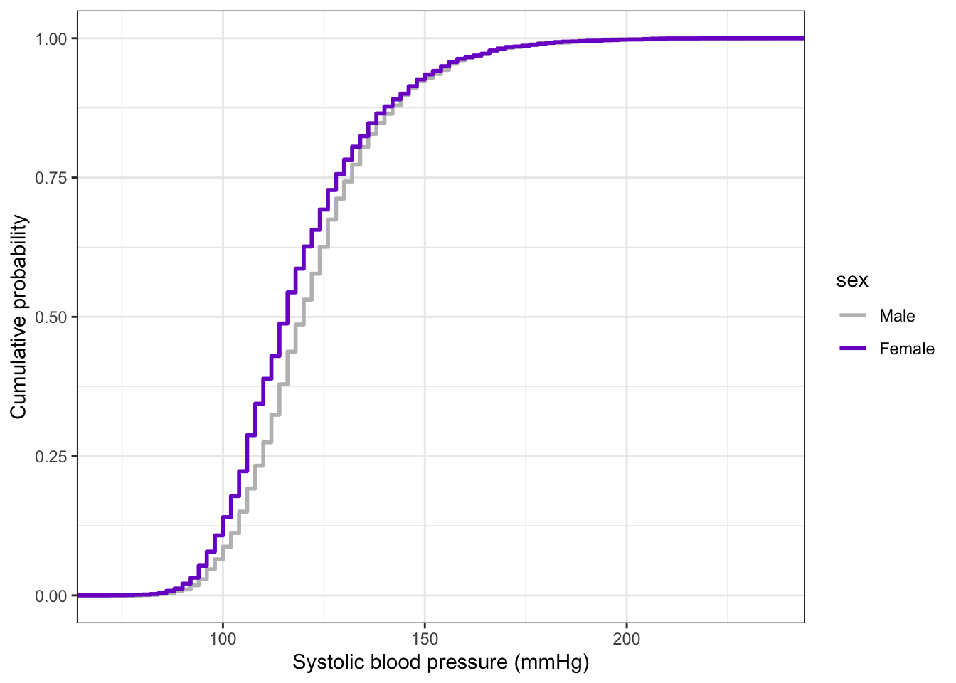
The test statistic, D, is the maximum distance between the two empirical cumulative distribution functions (ECDFs). ECDFs are a special type of probability distribution showing the cumulative probability of the values of a variable. We can examine the difference between the ECDFs for systolic blood pressure of males and females in the sample with the following graph:
R Code 6.61 : Compute empirical cumulative distributions (ECDFs)
Code
bp_clean|>ggplot2::ggplot(ggplot2::aes( x =systolic, color =sex))+ggplot2::stat_ecdf( geom ="step", linewidth =1, na.rm =TRUE)+ggplot2::labs( x ="Systolic blood pressure (mmHg)", y ="Cumulative probability")+ggplot2::scale_color_manual( values =c("Male"="gray", "Female"="purple3"))
Graph 6.13: ECDF of systolic blood pressure in mmHg by sex for 20152016 NHANES participants
At the widest gap between these two curves, males and females were \(.11\) apart, giving a test statistic of \(D = .11\).
Report
A K-S test comparing systolic blood pressure for males and females found a statistically significant difference between the two groups (D = .11; p < .05). This sample likely came from a population where the distribution of systolic blood pressure was different for males and females.
6.10.6 Miscellaneous
Resource 6.8 Miscellaneous packages for (possible) alternative tests
During my research for packages with functions for alternative test if the t-test assumption fail I came about several very interesting packages. Some of them work together with {ggplot2}, so that these statistics can be plotted easily as well.
{rcompanion}: I have outlined the table of content to demonstrate that this package contains many different tests. (See
{ggstats}: Provides new statistics, new geometries and new positions for {ggplot2} and a suite of functions to facilitate the creation of statistical plots.
{ggstatsplot}: As an extension of {ggplot2} the packages creates graphics with details from statistical tests included in the plots themselves.
{statsExpressions}: Tidy Data Frames and Expressions with Statistical Details. Utilities for producing data frames with rich details for the most common types of statistical approaches and tests.
Table 6.8: Download average numbers of miscellanous packages with test functions
The Anderson-Darling Goodness of Fit Test (AD-Test) is a measure of how well your data fits a specified distribution. It’s commonly used as a test for normality. (<a href="https://www.statisticshowto.com/anderson-darling-test/">Statistics How-To</a>)
Boxplots
Boxplots are a visual representation of data that shows central tendency (usually the median) and spread (usually the interquartile range) of a numeric variable for one or more groups; boxplots are often used to compare the distribution of a continuous variable across several groups. (SwR, Glossary)
Cohen’s d
Cohen’s d is a standardized effect size for measuring the difference between two group means. It is frequently used to compare a treatment to a control group. It can be a suitable effect size to include with t-test and ANOVA results. (<a href= "https://statisticsbyjim.com/basics/cohens-d/">Statistics by Jim</a>)
Degrees of Freedom
Degree of Freedom (df) is the number of pieces of information that are allowed to vary in computing a statistic before the remaining pieces of information are known; degrees of freedom are often used as parameters for distributions (e.g., chi-squared, F). (SwR, Glossary)
ECDF
In statistics, an empirical distribution function (commonly also called an empirical cumulative distribution function, eCDF) is the distribution function associated with the empirical measure of a sample. This cumulative distribution function is a step function that jumps up by 1/n at each of the n data points. Its value at any specified value of the measured variable is the fraction of observations of the measured variable that are less than or equal to the specified value. (<a href="https://en.wikipedia.org/wiki/Empirical_distribution_function">Wikipedia</a>) A CDF is a hypothetical model of a distribution, the ECDF models empirical (i.e. observed) data. (<a href="https://www.statisticshowto.com/empirical-distribution-function/">Statistics How To</a>)
Effect Size
Effect size is a measure of the strength of a relationship; effect sizes are important in inferential statistics in order to determine and communicate whether a statistically significant result has practical importance. (SwR, Glossary)
Homogeneity of Variances
Homogeneity of variances is equal variances among groups; homogeneity of variance is one of the assumptions tested for independent and dependent t-tests and analysis of variance. (SwR, Glossary)
Independent
Independent-samples t-test or unpaired sample t-test is an inferential test comparing two independent means. (SwR, Glossary)
Kolmogorov-Smirnov
The Kolmogorov-Smirnov test is used when the assumption of equal variances (homogeneity of variances) fails for the independent-samples t-test; the test compares the distributions of the groups rather than their means. (SwR, Glossary)
Kurtosis
Kurtosis is a measure of how many observations are in the tails of a distribution; distributions that look bell-shaped, but have a lot of observations in the tails (platykurtic) or very few observations in the tails (leptokurtic) (SwR, Glossary)
Leptokurtic
Leptokurtic is a distribution of a numeric variable that has many values clustered around the middle of the distribution; leptokurtic distributions often appear tall and pointy compared to mesokurtic or platykurtic distributions. (SwR, Glossary)
Mann-Whitney
Mann-Whitney U test, also called Wilcoxon rank sum test, is an alternative for comparing a numeric or ordinal variable across two groups when the independent-samples t-test assumption of normality is not met. (SwR, Glossary)
Omnibus
An omnibus is a statistical test that identifies that there is some relationship going on between variables, but not what that relationship is. (SwR, Glossary)
One-sample
One-sample t-test, also known as the single-parameter t-test or single-sample t-test, is an inferential statistical test comparing the mean of a numeric variable to a population or hypothesized mean. (SwR, Glossary)
Outcome
Outcome is the variable being explained or predicted by a model; in linear and logistic regression, the outcome variable is on the left-hand side of the equal sign. (SwR, Glossary)
p-value
The p-value is the probability that the test statistic is at least as big as it is under the null hypothesis (SwR, Glossary)
Paired
Dependent-samples test or paired-samples t-test is an inferential test comparing two related means . (SwR, Glossary)
Platykurtic
Platykurtic is a distribution of a numeric variable that has more observations in the tails than a normal distribution would have; platykurtic distributions often look flatter than a normal distribution. (SwR, Glossary)
Pooled Variance
Pooled variance is the assumption that the variances in two groups are equal, so these variances are combined ('pooled') (SwR, Glossary).
Predictor Variable
Predictor variable -- also known sometimes as the independent or explanatory variable -- is the counterpart to the response or dependent variable. Predictor variables are used to make predictions for dependent variables. ([DeepAI](https://deepai.org/machine-learning-glossary-and-terms/predictor-variable), [MiniTab](https://support.minitab.com/en-us/minitab/21/help-and-how-to/statistical-modeling/regression/supporting-topics/basics/what-are-response-and-predictor-variables/))
Q-Q-Plot
A quantile-quantile plot is a visualization of data using probabilities to show how closely a variable follows a normal distribution. (SwR, Glossary) This plot is made up of points below which a certain percentage of the observations fall. On the x-axis are normally distributed values with a mean of 0 and a standard deviation of 1. On the y-axis are the observations from the data. If the data are normally distributed, the values will form a diagonal line through the graph. (SwR, chapter 6)
Quantile
Quantiles are cut points dividing the range of a probability distribution into continuous intervals with equal probabilities (<a href="https://en.wikipedia.org/wiki/Quantile">Wikipedia</a>)
Rejection Region
Rejection region is the area under the curve of a sampling distribution where the probability of obtaining a value is very small, often below 5%; the rejection region is in the end of the tail or tails of the distribution. (SwR, Glossary)
Shapiro-Wilk
The Shapiro-Wilk test is a statistical test to determine or confirm whether a variable has a normal distribution; it is sensitive to small deviations from normality and not useful for sample sizes above 5,000 because it will nearly always find non-normality. (SwR, Glossary)
Sign-Test
Sign-test is a a statistical test that compares the median of a variable to a hypothesized or population value; used in lieu of the one-sample t-test when the t-test assumptions are not met. (SwR, Glossary)
Skewness
Skewness is the extent to which a variable has extreme values in one of the two tails of its distribution (SwR, Glossary)
Standard Deviation
The standard deviation is a measure of the amount of variation or dispersion of a set of values. A low standard deviation indicates that the values tend to be close to the mean (also called the expected value) of the set, while a high standard deviation indicates that the values are spread out over a wider range. The standard deviation is the square root of its variance. A useful property of the standard deviation is that, unlike the variance, it is expressed in the same unit as the data. Standard deviation may be abbreviated SD, and is most commonly represented in mathematical texts and equations by the lower case Greek letter $\sigma$ (sigma), for the population standard deviation, or the Latin letter $s$ for the sample standard deviation. ([Wikipedia]
Standard Error
The standard error (SE) of a statistic is the standard deviation of its [sampling distribution]. If the statistic is the sample mean, it is called the standard error of the mean (SEM). (<a href="https://en.wikipedia.org/wiki/Standard_error">Wikipedia</a>) The standard error is a measure of variability that estimates how much variability there is in a population based on the variability in the sample and the size of the sample. (SwR, Glossary)
T-Statistic
The T-Statistic is used in a T test when you are deciding if you should support or reject the null hypothesis. It’s very similar to a Z-score and you use it in the same way: find a cut off point, find your t score, and compare the two. You use the t statistic when you have a small sample size, or if you don’t know the population standard deviation. (<a href="https://www.statisticshowto.com/t-statistic/">Statistics How-To</a>)
Welch-T
Welch’s t-test is a variation on the Student’s t-test that does not assume equal variances in group (SwR, Glossary).
Wilcoxon
Wilcoxon signed-ranks test is an alternative to the dependent-samples t-test when the continuous variable is not normally distributed; it uses ranks to determine whether the values of a numeric variable are different across two related groups. (SwR, Glossary)
Z-score
A z-score (also called a standard score) gives you an idea of how far from the mean a data point is. But more technically it’s a measure of how many standard deviations below or above the population mean a raw score is. (<a href="https://www.statisticshowto.com/probability-and-statistics/z-score/#Whatisazscore">StatisticsHowTo</a>)
Delacre, Marie, Daniël Lakens, and Christophe Leys. 2017. “Why Psychologists Should by Default Use Welch’s t-Test Instead of Student’s t-Test” 30 (1): 92. https://doi.org/10.5334/irsp.82.
———. 2022. “Correction: Why Psychologists Should by Default Use Welch’s t-Test Instead of Student’s t-Test” 35 (1): 21. https://doi.org/10.5334/irsp.661.
# T-test {#sec-chap06}```{r}#| label: setup#| include: falsebase::source(file ="R/helper.R")ggplot2::theme_set(ggplot2::theme_bw()) ``````{r}#| label: cranlogs#| include: false#| eval: false## run only once manually #########cranlogs_cohensd <-pkgs_dl(c("lsr", "effectsize", "rstatix", "effsize"))save_data_file("chap06", cranlogs_cohensd, "cranlogs_cohensd.rds")cranlogs_skewness <-pkgs_dl(c("datawizard", "e1071", "moments", "psych", "semTools", "statpsych"))save_data_file("chap06", cranlogs_skewness, "cranlogs_skewness.rds")cranlogs_ad_test <-pkgs_dl(c("cmstatr", "DescTools", "kSamples", "nortest"))save_data_file("chap06", cranlogs_ad_test, "cranlogs_ad_test.rds")cranlogs_levene_test <-pkgs_dl(c("car", "DescTools", "misty", "rstatix"))save_data_file("chap06", cranlogs_levene_test, "cranlogs_levene_test.rds")cranlogs_sign_test <-pkgs_dl(c("BSDA", "DescTools", "rstatix"))save_data_file("chap06", cranlogs_sign_test, "cranlogs_sign_test.rds")cranlogs_misc <-pkgs_dl(c("ggstats", "ggstatsplot", "rcompanion", "statsExpressions"))save_data_file("chap06", cranlogs_misc, "cranlogs_misc.rds")```## Achievements to unlock:::::: {#obj-chap06}::::: my-objectives::: my-objectives-headerObjectives for chapter 06:::::: my-objectives-container**SwR Achievements**- **Achievement 1**: Understanding the relationship between one categorical variable and one continuous variable using histograms, means, and standard deviations (@sec-chap06-achievement1)- **Achievement 2**: Comparing a sample mean to a population mean with a `r glossary("one-sample", "one-sample t-test")` (@sec-chap06-achievement2)- **Achievement 3**: Comparing two unrelated sample means with an `r glossary("independent", "independent-samples t-test")` (@sec-chap06-achievement3)- **Achievement 4**: Comparing two related sample means with a `r glossary("paired", "dependent-samples t-test")` (@sec-chap06-achievement4)- **Achievement 5**: Computing and interpreting an `r glossary("effect size")` for significant t-tests (@sec-chap06-achievement5)- **Achievement 6**: Examining and checking the underlying assumptions for using the t-test (@sec-chap06-achievement6)- **Achievement 7**: Identifying and using alternate tests when t-test assumptions are not met (@sec-chap06-achievement7)::::::::Achievements for chapter 06::::::## The blood pressure predicament- **Systolic blood pressure** is measured in millimeters of mercury, or mmHG, and ranges from 74 to 238.- **Diastolic blood pressure** is also measured in mmHG and ranges from 0 to 120.## Resources & Chapter Outline### Data, codebook, and R packages {#sec-chap04-data-codebook-packages}:::::: my-resource:::: my-resource-header::: {#lem-chap06-resources}: Data, codebook, and R packages for learning about t-test:::::::::: my-resource-container**Data**Two options for accessing the data:- Download the data set `nhanes_2015–2016_ch6.csv` from <https://edge.sagepub.com/harris1e>.- Follow the instructions in Box 6.1 to import the data directly with the halp of {**NHANES**} from the Internet into R.**Codebook**Two options for accessing the codebook:- Download the codebook files `nhanes_demographics_20152016_codebook.html` and `nhanes_examination_20152016_codebook.html` from <https://edge.sagepub.com/harris1e>.\- Use the online version of the codebook on the NHANES website (https://www.cdc.gov/nchs/nhanes/index.htm)**Packages**1. Packages used with the book (sorted alphabetically)- {**BSDA**} @sec-BSDA (Alan T. Arnholt)- {**car**} @sec-car (John Fox)- {**lsr**} @sec-lsr (Danielle Navarro)\- {**rcompanion**} 1 (Salvatore Mangiafico)- {**RNHANES**} @sec-RNHANES (Herb Susmann)- {**tidyverse**}: @sec-tidyverse (Hadley Wickham)2. My additional packages new introduced (sorted alphabetically)- {**datawizard**} @sec-datawizard (Etienne Bacher)- {**e1071**} @sec-e1071 (David Meyer)- {**effectsize**} @sec-effectsize (Mattan S. Ben-Shachar)- {**moments**} @sec-moments (Lukasz Komsta)- {**misty**} @sec-misty (Takuya Yanagida)- {**nhanesA**} @sec-nhanesA (Christopher Endres)- {**nortest**} @sec-nortest (Uwe Ligges)- {**psych**} @sec-psych (William Revelle)- {**rcompanion**} 1 (Salvatore Mangiafico):::::::::### Get data::::::::::::::: my-example:::: my-example-header::: {#exm-chap06-get-data}: Numbered Example Title::::::::::::::::::: my-example-container::::::::::: panel-tabset###### NHANES data:::::: my-r-code:::: my-r-code-header::: {#cnj-chap06-get-nhanes-data}: Get NHANES data for blood pressure examination with demographics variable for 2015-2016:::::::::: my-r-code-container```{r}#| label: get-nhanes-data#| cache: true#| eval: false## run one once manually ########### list EXAM tables for 2016 to get file namesexam_tables_2016 <- nhanesA::nhanesTables('EXAM', 2016)## list variables in BPX_I (Blood Pressure file)bpx_i_variables <- nhanesA::nhanesTableVars('EXAM', 'BPX_I')bpx_i <- nhanesA::nhanes('BPX_I')demo_i <- nhanesA::nhanes('DEMO_I')bpx_2016 <- dplyr::full_join(demo_i, bpx_i, by ="SEQN")save_data_file("chap06", bpx_2016, "bpx_2016.rds")```(*For this R code chunk is no output available. For the raw data see* ):::::::::###### NHANES codebook:::::: my-r-code:::: my-r-code-header::: {#cnj-chap06-get-nhanes-codebook}: Get NHANES codebook for blood pressure examination with demographics variable for 2015-2016:::::::::: my-r-code-container```{r}#| label: get-nhanes-codebookcb_systolic <- nhanesA::nhanesCodebook("BPX_I", "BPXSY1")cb_diastolic <- nhanesA::nhanesCodebook("BPX_I", "BPXDI1")```------------------------------------------------------------------------(*For this R code chunk is no output available. For the raw data see*)Besides to call the appropriate website for 2015-2016 [examination codebook](nhanes_examination_20152016_codebook.html) and [demographic codebook](nhanes_demographics_20152016_codebook.html) there is also the option to download information via {**nhanesA**}.:::::::::::::::::::::::::::::::::::::::::::::::------------------------------------------------------------------------### Show raw data:::::::::::::::: my-example:::: my-example-header::: {#exm-chap06-show-raw-data}: Numbered Example Title:::::::::::::::::::: my-example-container:::::::::::: panel-tabset###### Blood pressure data::::::: my-r-code:::: my-r-code-header::: {#cnj-chap06-glance-nhanes-data}: Glance at NHANES data for blood pressure examination with demographics variable for 2015-2016::::::::::: my-r-code-container::: {#lst-glance-nhanes-data}```{r}#| label: glance-nhanes-databpx_2016 <- base::readRDS("data/chap06/bpx_2016.rds")skimr::skim(bpx_2016)my_glance_data(bpx_2016)```Glance at NHANES data for blood pressure examination with demographics variable for 2015-2016::::::::::::::###### Blood pressure codebook:::::: my-r-code:::: my-r-code-header::: {#cnj-chap06-glance-nhanes-codebook}: Glance at NHANES codebook for systolic & diastolic blood pressure (2015-2016):::::::::: my-r-code-container```{r}#| label: glance-nhanes-codebook#| results: holdglue::glue("*********************** Systolic blood pressure ******************")cb_systolicglue::glue(" ")glue::glue("*********************** Diastolic blood pressure ******************")cb_diastolic```::::::::::::::::::::::::::::::::::::::::::::::::::------------------------------------------------------------------------### Recode data:::::: my-r-code:::: my-r-code-header::: {#cnj-chap06-clean-data}: Clean NHANES blood pressure data (2015-2016):::::::::: my-r-code-container```{r}#| label: clean-data## load bpx_2016 #######bpx_2016 <- base::readRDS("data/chap06/bpx_2016.rds")bp_clean <- bpx_2016 |> dplyr::rename(systolic = BPXSY1,systolic2 = BPXSY2,sex = RIAGENDR ) |> dplyr::mutate(diff_syst = systolic - systolic2) |> dplyr::relocate(c(systolic, systolic2, diff_syst), .before = sex)save_data_file("chap06", bp_clean, "bp_clean.rds")```------------------------------------------------------------------------(*For this R code chunk is no output available*):::::::::## Achievement 1: Relationship between one categorical and one continuous variable {#sec-chap06-achievement1}For this first achievement we are going to look into the relationship between one categorical variable and one continuous variable using histograms, means, and standard deviations.::::::::::::::::::::::::::: my-example:::: my-example-header::: {#exm-chap06-descriptive}: Description of blood pressure data from NHANES 2015-2016::::::::::::::::::::::::::::::: my-example-container::::::::::::::::::::::: panel-tabset###### Histogram 1:::::: my-r-code:::: my-r-code-header::: {#cnj-chap06-systolic-histo1}: Histogram of systolic blood pressure (NHANES 2015-2016):::::::::: my-r-code-container```{r}#| label: systolic-histo1#| fig-cap: "Histogram of systolic blood pressure (NHANES 2015-2016)"## load bpx_2016 #######bpx_2016 <- base::readRDS("data/chap06/bpx_2016.rds")## graph systolic blood pressure variable BPXSY1 (Figure 6.1)sys_histo <- bpx_2016 |> ggplot2::ggplot( ggplot2::aes(x = BPXSY1) ) + ggplot2::geom_histogram(fill ="mediumpurple",color ="white",bins =30,na.rm =TRUE ) + ggplot2::theme_bw() + ggplot2::labs(x ="Systolic blood pressure (mmHg)", y ="NHANES participants" ) sys_histo```------------------------------------------------------------------------This is the replication of the book’s Figure 6.1.The graph is not exactly normally distributed; it has a little right skew. The `r glossary("quantile")` values (0% 25% 50% 75% 100%) are `r quantile(bpx_2016$BPXSY1, na.rm = TRUE)`. The middle 50% lies in the range between `r quantile(bpx_2016$BPXSY1, 0.25, na.rm = TRUE)` and `r quantile(bpx_2016$BPXSY1, 0.75, na.rm = TRUE)` mmHG. You can't see the highest values because their frequencies are too small.:::::::::###### Histogram 2:::::: my-r-code:::: my-r-code-header::: {#cnj-chap06-systolic-histo2}: Histogram of systolic blood pressure with risk factors (NHANES 2015-2016):::::::::: my-r-code-container```{r}#| label: systolic-histo2#| fig-cap: "Histogram of systolic blood pressure with risk factors (NHANES 2015-2016)"## graph systolic blood pressure with risk factors (Figure 6.2)sys_histo2 <- bpx_2016 |> ggplot2::ggplot( ggplot2::aes(x = BPXSY1, fill = BPXSY1 >120) ) + ggplot2::geom_histogram(color ="white",bins =30,na.rm =TRUE) + ggplot2::theme_bw() + ggplot2::labs(x ="Systolic blood pressure (mmHg)", y ="NHANES participants" ) + ggplot2::scale_fill_manual(values =c("mediumpurple", "grey"),labels =c("Normal range","at-risk or high"),name ="Systolic\nBlood Pressure" )sys_histo2```------------------------------------------------------------------------This is the replication of the book’s Figure 6.2.:::::::::###### Experiment:::::: my-r-code:::: my-r-code-header::: {#cnj-chap06-systolic-histo3}: Blood pressure histogram with several colors according to their medical conditions:::::::::: my-r-code-container```{r}#| label: systolic-histo3## graph systolic blood pressure differentiatedsys_histo3 <- bpx_2016 |> dplyr::select(BPXSY1) |> dplyr::mutate(sys = dplyr::case_when( BPXSY1 <105~"0", BPXSY1 >=105& BPXSY1 <120~"1", BPXSY1 >=120& BPXSY1 <130~"2", BPXSY1 >=130& BPXSY1 <140~"3", BPXSY1 >=140~"4" ) ) |> ggplot2::ggplot( ggplot2::aes(x = BPXSY1, fill = sys) ) + ggplot2::geom_histogram(color ="white",binwidth =2,na.rm =TRUE) + ggplot2::theme_bw() + ggplot2::theme(legend.position ="bottom") + ggplot2::labs(x ="Systolic blood pressure (mmHg)", y ="NHANES participants" ) + ggplot2::scale_fill_manual(values =c("0"="grey", "1"="mediumpurple", "2"="yellow", "3"="darkorange", "4"="red" ),labels =c("Low","Optimal","Normal","At-risk","High" ),name ="Systolic\nBlood Pressure" ) + ggplot2::xlim(70, 240)sys_histo3```------------------------------------------------------------------------Here I have experimented to colorize the histogram with different colors. I took as borders the medical condition for isolated blood pressure measures:- Low: \< 105- Optimal: \>= 105 & \< 120- Normal: \>= 120 & \< 130- At Risk: \>= 130 & \< 140- High: \>= 140In this case I can’t use the color directly as `fill` variable into the `ggplots::aes()` function. Besides I learned two other solve two other issues:- The sequence of colors are aligned to the values alphabetically. Therefore I had to take characters that are sorted in the correct order. I took c("0", "1", "2", "3", "4") but c("a", "b", "c", "d" ,"e") would have worked too.- Wider bins brought the problem that the color has changed in the middle of the bar length. I did not know how to solve this issue generally, for instance with providing `breaks` or to provide borders conforming to the medical status. Only `binwidth` of 1 and 2 worked, 3 already showed the problem. Other people had the same problem, see for instance the section "Example 2: Draw Histogram with Different Colors Using ggplot2 Package" in [Draw Histogram with Different Colors in R (2 Examples)](https://statisticsglobe.com/draw-histogram-with-different-colors-in-r)[@schorkn.d].:::::::::###### Histogram 3:::::: my-r-code:::: my-r-code-header::: {#cnj-chap06-diastolic-histo}: Histogram of diastolic blood pressure with risk factors (NHANES 2015-2016):::::::::: my-r-code-container```{r}#| label: diastolic-histo#| fig-cap: "Histogram of diastolic blood pressure with risk factors (NHANES 2015-2016)"## graph systolic blood pressure with risk factors (Figure 6.3)dia_histo <- bpx_2016 |> ggplot2::ggplot( ggplot2::aes(x = BPXDI1, fill = BPXDI1 >80) ) + ggplot2::geom_histogram(color ="white",bins =30,na.rm =TRUE) + ggplot2::theme_bw() + ggplot2::labs(x ="Diastolic blood pressure (mmHg)", y ="NHANES participants" ) + ggplot2::scale_fill_manual(values =c("mediumpurple", "grey"),labels =c("Normal range","at-risk or high"),name ="Diastolic\nBlood Pressure" )dia_histo```------------------------------------------------------------------------This is the replication of the book’s Figure 6.3.:::::::::###### `mean()` & `sd()`:::::: my-r-code:::: my-r-code-header::: {#cnj-chap06-systolic-mean-sd}: Mean and standard deviation of systolic blood pressure in the NHANES data sample (2015-2016):::::::::: my-r-code-container```{r}#| label: systolic-mean-sdbpx_stats <- bpx_2016 |> tidyr::drop_na(BPXSY1) |> dplyr::summarize(mean = base::mean(BPXSY1),sd = stats::sd(BPXSY1),n = dplyr::n() )bpx_stats```:::::::::::::::::::::::::::::::::::::::::::::::::::::::::::::::::::::::::::::::::::## Achievement 2: One-Sample t-test {#sec-chap06-achievement2}### IntroductionWe have a mean of the systolic blood pressure a little bit above 120.54 mmHG. This is almost exactly the upper cutoff value of 120 mmHG for the "normal range" of blood pressure. Is this only valid for the sample of also for the whole population? Have about half of the US people high systolic blood pressure, e.g. more than 120mmHG? The question can be answered with a `r glossary("one-sample", "one-sample t-test")`. The one sample t-test compares a sample mean to a *hypothesized or population* mean.::::: my-important::: my-important-headerThere are three different t-tests:::::: my-important-container- **One-sample t-test**: compares a mean to a population or hypothesized value- **Independent-samples t-test**: compares the means of two unrelated groups- **Dependent-samples t-test**: compares the means of two related groups::::::::The t-distribution has a bell shape like the normal distribution. But unlike the normal distribution its variance is not known but approximated with its only parameter `r glossary("degrees of freedom")` (df). `df` is calculated by the number of observations minus one ($n-1$). With higher degrees of freedom the t-distribution will get closer to the normal distribution. Often the number 30 is recommended as the cutting point where t-distribution and normal distribution are equivalent.I am following @prp-chap05-nhst from @sec-chap05-achievement5.### NHST Step 1Write the null and alternate hypotheses:Two considerations:1. The Null relates most of the times to a situation where no change occurs. In this case that there is no difference in the means of the systolic blood pressure. This is different to the assumption that the mean difference is not higher than 120 mmHG!2. In the one-sample t-test we are comparing sample mean with population mean. In this case the NHANES sample from the 2015-2016 data with the population mean of the US population.::: callout-note- **H0**: There is no difference in the mean systolic blood pressure in the US population and the cutoff for normal blood pressure of 120 mmHG in the NHANES 2015-2016 data set.- **HA**: There is a difference in the mean systolic blood pressure in the US population and the cutoff for normal blood pressure of 120 mmHG in the NHANES 2015-2016 data set.:::### NHST Step 2Compute the test statistic. The one-sample t-test uses the `r glossary("t-statistic")` (sort of like a z-statistic):::::: my-theorem:::: my-theorem-header::: {#thm-chap06-t-statistic}: t-test formula:::::::::: my-theorem-container$$t = \frac{m_{x} - \mu_{x}}{\frac{s_x}{\sqrt{n_{x}}}}$$ {#eq-chap06-t-statistic}- $m_{x}$ represents the mean of the variable x, the variable to be tested,- $\mu_{x}$ is the *population mean or hypothesized value* of the variable,- $s_{x}$ is the sample standard deviation of x, and- $n_{x}$ is the sample size:::::::::The formula is very similar as the `r glossary("Z-score")` statistic in @eq-chap04-z-score. The only difference is that in the above `r glossary("t-statistic")` the denominator is the `r glossary("standard deviation")` rather than the `r glossary("standard error")`.- `z` shows how many sample standard deviations some value is away from the mean.- `t` shows how many standard errors (i.e., population standard deviations) some value is away from the mean.$$t = \frac{120.5394 - 120}{\frac{18.61692}{\sqrt{7145}}} = 2.45$$:::::: my-r-code:::: my-r-code-header::: {#cnj-chap06-t-statistic-systolic}: t-statistic of systolic blood pressure aof NHANES sample with hypothesized population mean:::::::::: my-r-code-container```{r}#| label: t-statistic-systolic( t_test_systolic <- stats::t.test( bpx_2016$BPXSY1,alternative ="two.sided",mu =120))## for later use #########t_sys = t_test_systolic[["statistic"]][["t"]]df_sys = t_test_systolic[["parameter"]][["df"]]null_sys = t_test_systolic[["null.value"]][["mean"]]estimate_sys = t_test_systolic[["estimate"]][["mean of x"]]p_value_sys = t_test_systolic[["p.value"]]se_sys = t_test_systolic[["stderr"]]```------------------------------------------------------------------------I have stored the result of the t-test into variables for later use.::::::::::::::: my-assessment:::: my-assessment-header::: {#cor-chap06-t-test-output}: Explications of the t-test output:::::::::: my-assessment-container**1. Line**: Data (variable) used. **2. Line**: - `t`: value of the t-test statistic. - `df`: degrees of freedom, with t-statistic = subtracting 1 from sample size = $n - 1$. - `p-value`: The probability of the sample coming from a population where the null hypothesis is true. **3. Line**: wording of the alternative hypothesis. **4. Line**: Chosen confidence interval. **5. Line**: The lower and upper boundary of the confidence interval. **6. Line**: Sample estimates that has to be compared to the value of the null hypothesis.:::::::::### NHST Step 3Review and interpret the test statistics: Calculate the probability that your test statistic is at least as big as it is if there is no relationship (i.e., the null is true).The following examples replicates Figure 6.4, 6.5 and 6.6. I will break down the final code into several steps following the nice article \[Visualizing Sampling Distributions: Learn how to add areas under the curve in sampling distributions\]https://ggplot2tutor.com/tutorials/sampling_distributions [@burkhart2021].::::::::::::::::::::::::::::::::::: my-example:::: my-example-header::: {#exm-chap06-prob-dist-t-test}: Probability distribution of t-test statistic::::::::::::::::::::::::::::::::::::::: my-example-container::::::::::::::::::::::::::::::: panel-tabset###### t (df=1):::::: my-r-code:::: my-r-code-header::: {#cnj-chap06-two-t-prob-dist}: Student t distributions with 1 degree of freedom (df):::::::::: my-r-code-container```{r}#| label: fig-t-prob-dist#| fig-cap: Student t distributions with 1 degree of freedom (df)ggplot2::ggplot() + ggplot2::xlim(-7, 7) +## or as an alternative# ggplot2::ggplot(tibble::tibble(x = c(-7, 7)), # ggplot2::aes(x)) + ggplot2::stat_function(fun = stats::dt,args =list(df =1),geom ="line",linewidth =0.7 ) + ggplot2::theme_bw()```::::::::::::::: my-procedure:::: my-procedure-header::: {#prp-chap06-plot-dist}: Plotting a distribution with {**ggplot2**}:::::::::: my-procedure-container1. As there is no data (just the formula for the function) we need to specify the x-limits.2. `ggplot2::stat_function` draws the function. We can specify the function extra or create an anonymous function or --- as I have done here --- use a function from an R package. Note that there is no parenthesis behind the function name.:::::::::###### comparing t:::::: my-r-code:::: my-r-code-header::: {#cnj-chap06-compare-t-prob-dist}: Student t distributions with 1 and 7144 degree of freedom (df) and normal distribution compared:::::::::: my-r-code-container```{r}#| label: fig-compare-t-prob-dist#| fig-cap: Student t distributions with 1 and 7144 degree of freedom (df) and normal distribution comparedggplot2::ggplot(tibble::tibble(x =c(-7, 7)), ggplot2::aes(x)) + ggplot2::stat_function(fun = stats::dt,args =list(df =1),geom ="line",linewidth =0.7, ggplot2::aes(linetype ="1") ) + ggplot2::stat_function(fun = stats::dt,args =list(df =7144),geom ="line",linewidth =0.7, ggplot2::aes(linetype ="5") ) + ggplot2::stat_function(fun = stats::dt,args =list(df =30),geom ="line",linewidth =0.7, ggplot2::aes(linetype ="3") ) + ggplot2::stat_function(fun = stats::dnorm,geom ="line",linewidth =0.7, ggplot2::aes(color ="red") ) + ggplot2::scale_linetype_discrete(name ="t dist",labels =c("df = 1", "df = 30", "df = 7144") ) + ggplot2::scale_color_discrete(name ="normal dist",labels ="mean = 0, sd = 1" ) + ggplot2::theme_bw()```------------------------------------------------------------------------The plot shows two things:1. There is a big difference between a t distribution with df = 1 and df = 30.2. There is no visible difference between t with df = 30, df = 7144 and a normal distribution.::::::::::::::: my-procedure:::: my-procedure-header::: {#prp-chap06-plot-several-dist}: Plotting several distributions with {**ggplot2**}:::::::::: my-procedure-container1. Use for every distribution `ggplot2::stat_function()`.2. Put the aesthetic into an `ggplot2::aes()` function.3. Add for each legend a corresponding scale with name and labels.:::::::::###### t systolic:::::: my-r-code:::: my-r-code-header::: {#cnj-code-name-b}: t-distribution (df = 7,144) shaded for values of 2.4491 or higher (replicating Figure 6.5):::::::::: my-r-code-container```{r}#| label: fig-t-test-systolic#| fig-cap: "t-distribution (df = 7,144) shaded for values of 2.4491 or higher (replicating Figure 6.5)"ggplot2::ggplot() + ggplot2::xlim(-4, 4) + ggplot2::stat_function(fun = stats::dt,args =list(df = df_sys),geom ="line",linewidth =0.7 ) + ggplot2::stat_function(fun = stats::dt,args =list(df = df_sys),geom ="area",xlim =c(t_sys, 4), ggplot2::aes(fill =paste("t >=", round(t_sys, 3)) ) ) + ggplot2::theme_bw() + ggplot2::scale_fill_manual(name ="",values ="steelblue" )```------------------------------------------------------------------------The plot shows that the t-value of 2.499 is very unlikely if the null hypotheses were true, e.g. if the sample comes from a population with a systolic blodd pressure mean of 240.:::::::::###### 2.5% shaded:::::: my-r-code:::: my-r-code-header::: {#cnj-chap06-two-sided-shaded}: t-distribution (df = 7,144) with 2.5% shaded in each tail of the distribution (replicating Figure 6.6):::::::::: my-r-code-container```{r}#| label: fig-two-sided-shaded#| fig-cap: "t-distribution (df = 7,144) with 2.5% shaded in each tail of the distribution (replicating Figure 6.6)"ggplot2::ggplot() + ggplot2::xlim(-4, 4) + ggplot2::stat_function(fun = stats::dt,args =list(df = df_sys),geom ="line",linewidth =0.7 ) + ggplot2::stat_function(fun = stats::dt,args =list(df = df_sys),geom ="area",xlim =c(1.96, 4), ggplot2::aes(fill =paste("Rejection region") ) ) + ggplot2::stat_function(fun = stats::dt,args =list(df = df_sys),geom ="area",xlim =c(-4, -1.96), ggplot2::aes(fill =paste("Rejection region") ) ) + ggplot2::theme_bw() + ggplot2::scale_fill_manual(name ="",values ="purple3" ) + ggplot2::labs(x ="t-statistic",y ="Probability density" )```------------------------------------------------------------------------The plot shows the rejection regions for the probability of 95%.$$\begin{align*}p_{low}(x > 1.96) \approx 0.025 \\p_{high}(x < 1.96) \approx 0.975 \\p_{high} - p_{low} = \\0.975 - 0.025 = 0.95\end{align*}$$:::::::::###### t systolic & 2.5% shaded overlaid:::::: my-r-code:::: my-r-code-header::: {#cnj-chap06-t-two-sided-shaded}: t-distribution (df = 7,144) with 2.5% shaded in each tail of the distribution (replicating Figure 6.6):::::::::: my-r-code-container```{r}#| label: fig-t-two-sided-shaded#| fig-cap: "t-distribution (df = 7,144) with 2.5% shaded in each tail of the distribution (replicating Figure 6.6)"ggplot2::ggplot() + ggplot2::xlim(-4, 4) + ggplot2::stat_function(fun = stats::dt,args =list(df = df_sys),geom ="line",linewidth =0.7 ) + ggplot2::stat_function(fun = stats::dt,args =list(df = df_sys),geom ="area",xlim =c(1.96, 4),alpha =0.5, ggplot2::aes(fill =paste("Rejection region"), ) ) + ggplot2::stat_function(fun = stats::dt,args =list(df = df_sys),geom ="area",xlim =c(-4, -1.96),alpha =0.5, ggplot2::aes(fill =paste("Rejection region"), ), ) + ggplot2::stat_function(fun = stats::dt,args =list(df = df_sys),geom ="area",xlim =c(t_sys, 4),alpha =0.5, ggplot2::aes(fill =paste("t >=", round(t_sys, 3)) ) ) + ggplot2::theme_bw() + ggplot2::scale_fill_manual(name ="",values =c("purple3", "red") ) + ggplot2::labs(x ="t-statistic",y ="Probability density" )```------------------------------------------------------------------------The plot shows that the t-value is in the `r glossary("rejection region", "rejection area")`, e.g., the null has to be rejected.:::::::::::::::::::::::::::::::::::::::::::::::::::::::::::::::::::::::::::::::::::::::::::::::::::::::::::### NHST Step 4Conclude and write the report.Even though the difference between the mean systolic blood pressure of `r round(estimate_sys, 2)` and the hypothesized value of `r null_sys` is small, it is statistically significant. The probability of this sample that it comes from a population where the mean systolic blood pressure is actually `r null_sys` is just `r round(p_value_sys, 3)*100`%. This sample is likely to be from a population with a higher mean blood pressure.::: callout-tipThe mean systolic blood pressure in a sample of `r df_sys + 1` people was `r round(estimate_sys, 2)` (sd = `r round(bpx_stats$sd, 2)`). A one-sample t-test found this mean to be statistically significantly different from the hypothesized mean of `r null_sys`\[t(`r df_sys`) = `r round(t_sys, 3)`; p = `r round(p_value_sys, 3)`\]. The sample likely came from a population with a mean systolic blood pressure not equal to `r null_sys`.:::## Achievement 3: Independent-samples t-test {#sec-chap06-achievement3}Instead of comparing one mean to a hypothesized or population mean, the `r glossary("independent", "independent-samples t-test")` compares the means of two groups to each other.We could for instance be interested to see if the blood pressure for persons of different sex are the same. Or the question statistically formulated: Do males and females in the sample come from a population where males and females have the same mean systolic blood pressure?I am not going into the details of achievement 3 because there is no much difference between the procedure for the one-sample t-test and the independent-samples t-test. Essentially there are only two differences:### Formula:::::: my-theorem:::: my-theorem-header::: {#thm-chap06-t-independent-test}: Independent-samples t-test formula:::::::::: my-theorem-container$$t = \frac{m_{1} - m_{2}}{\sqrt{\frac{s_1^2}{n_{1}} + \frac{s_2^2}{n_{2}}}}$$ {#eq-chap06-t-independent-test}- $m_{1}$ represents the mean of one group,- $m_{2}$ represents the mean of another group,- $s_{1}^2$ is the variance of the first group,- $s_{2}^2$ is the variance of the second group,- $n_{1}$ is the size of the first group,- $n_{2}$ is the size of the second group.:::::::::### Computing::::::: my-r-code:::: my-r-code-header::: {#cnj-chap06-t-indpendent-test}: Independent-samples t-test for systolic blood pressure of males and females::::::::::: my-r-code-container::: {#lst-chap06-t-indpendent-test}```{r}#| label: t-independent-test#| results: holdbp_clean = base::readRDS("data/chap06/bp_clean.rds")bp_clean |> tidyr::drop_na(systolic) |> dplyr::group_by(sex) |> dplyr::summarize(mean_systolic =mean(systolic),var_systolic =var(systolic),sample_size = dplyr::n() )two_sample_t <-t.test(formula = bp_clean$systolic ~ bp_clean$sex)two_sample_t```Independent-samples t-test for systolic blood pressure of males and females::::::::::::::It is important to note that category variables like `sex` do not work with the default `x, y` version of the t-test. Therefore we have to apply the method with class `formula`.In R formulae a single variable on the left-hand side is followed by the tilde sign `~` and one ore more objects that predict or explain the left-hand side.> In a lot of statistical tests, the object on the left-hand side of the formula is the `r glossary("outcome")` or dependent variable while the object(s) on the right-hand side of the formula are the `r glossary("predictor variable", "predictors")` or independent variables. (SwR)> It is commonly used to generate *design matrices* for modeling function (e.g. `lm`) [@kuhn2017].In our case, systolic blood pressure is the *outcome* being explained by the *predictor* of sex.In R the default t-test for independent samples is the `r glossary("Welch-T", "Welch’s t-test")` and not the student t-test.> Welch’s t-test is slightly different from the original formula for t, which used pooled variance in the denominator. `r glossary("Pooled variance")` assumes that the variances in the two groups are equal and combines them. (SwR)There is an scientific article explaining why Welch's t-test should be used in any case, even if the assumption of homogeneity of variance is met:> We show that the Welch’s t-test provides a better control of Type 1 error rates when the assumption of homogeneity of variance is not met, and it loses little robustness compared to Student’s t-test when the assumptions are met. We argue that Welch’s t-test should be used as a default strategy. [@delacre2017; see also: @delacre2022]Just to conclude this abbreviated section I quote the final summary reporting the independent t-test results.::: callout-tip> There was a statistically significant difference \[t(7143) = 7.31; p \< .05\] in mean systolic blood pressure between males (m = 122.18) and females (m = 118.97) in the sample. The sample was taken from the U.S. population, indicating that males in the United States likely have a different mean systolic blood pressure than females in the United States. The difference between male and female mean systolic blood pressure was 3.21 in the sample; in the population this sample came from, the difference between male and female mean blood pressure was likely to be between 2.35 and 4.07 (d = 3.21; 95% CI: 2.35–4.07). (SwR):::## Achievement 4: Dependent-samples t-test {#sec-chap06-achievement4}Again: I am not going to summarize this section because it resembles achievement 2 (one-sample t-test) and achievement 3 (independent.samples t-test).### Formula:::::: my-theorem:::: my-theorem-header::: {#thm-chap06-t-dependent-test}: Independent-samples t-test formula:::::::::: my-theorem-container$$t = \frac{m_{d} - 0}{\sqrt{\frac{s_d}{n_{d}}}}$$ {#eq-chap06-t-dependent-test}- $m_{d}$ represents the mean of differences between to measures,- $s_{d}^2$ is the variance of the mean differences between to measures,- $n_{d}$ is the sample size,- $0$ subtracting represents the null hypothesis; zero is the mean difference if the two measures were exactly the same.:::::::::### Computing::::: my-important::: my-important-headerGeneral advice before starting a test statistics:::::: my-important-containerAlways look at some visuals and descriptive statistics before you are starting the test procedure and following the NHST procedure as outlined in @prp-chap05-nhst.::::::::This shows that the *difference of the mean* between two measures is very small (0.55 mmHG). But it turned out that this value is highly statistically significant. But from a clinical point of view it is irrelevant!::::: my-important::: my-important-headerStatistically significant != meaningful!:::::: my-important-containerAll our three t-tests result in small but statistically significant values. This is an important reminder that statistically significant p-values are not necessarily of relevance.By the way: The reason for our small but statistically significant values are very large samples.::::::::The computation in R is the same as in @lst-chap06-t-indpendent-test. Again apply the formula version of Welch’s t-test with the only difference to add the argument `paired = TRUE`.## Achievement 5: Effect size {#sec-chap06-achievement5}### IntroductionWe haven seen that even the very small difference of 0.54 mmHG systolic blood pressure is with a large sample size statistically significant. But this small difference is clinically not relevant. To judge the importance of some statistically significant results we need effect sizes as another criteria.The proportion of people that believe that effect sizes are even more important than p-values is rising. P-values only report whether a difference or relationship from a sample is likely to be true in the population, while effect sizes provide information about the strength or size of a difference or relationship.In @sec-chap05 we discussed for the Chi-squared test as effect sizes- Cramèrs V (@sec-chap05-cramers-v)- Phi coefficient $\phi$ (@sec-chap05-phi-coefficient) and- Odds ratio (@sec-chap05-odds-ratio)For t-test the appropriate effect size measure is `r glossary("Cohen’s d")`.:::::: my-resource:::: my-resource-header::: {#lem-chap06-effect-size-assessment}Delving into effect size assessment:::::::::: my-resource-containerDerived from the importance of effect size parameter I need to know more how to use and interpret different kind of effect sizes. What follows are some resources- [Effect Size](https://en.wikipedia.org/wiki/Effect_size) (Wikipedia)- [Effect size](https://www.psy.gla.ac.uk/~steve/best/effect.html)[@draper2023]- [Effect size calculator](https://www.ai-therapy.com/psychology-statistics/effect-size-calculator) (AI-Therapie Statistics)- [Rules of thumb on magnitudes of effect sizes](https://imaging.mrc-cbu.cam.ac.uk/statswiki/FAQ/effectSize) (MRC Cognition and Brain Sciences Unit, University of Cambridge)- [Computation of Effect Sizes](https://www.psychometrica.de/effect_size.html)[@lenhard2022]::::::::::::::: my-theorem:::: my-theorem-header::: {#thm-chap06-cohens-d}: Formula for Cohen’s d one-sample t-test:::::::::: my-theorem-container$$d = \frac{m_{x} - \mu_{x}}{s_{x}}$$ {#eq-chap06-cohens-d-one-sample}$m_{x}$ = sample mean for $x$ $\mu_{x}$ = hypothesized or population mean $s_{x}$ = sample standard deviation for $x$:::::::::The formula is similar to the already well-known z-score calculation (@eq-chap04-z-score).:::::: my-assessment:::: my-assessment-header::: {#cor-chap06-cohens-d}: Classification of Cohen’s d values:::::::::: my-assessment-container- **Small effect size**: Cohen’s d = .2 to d \< .5- **Medium effect size**: Cohen’s d = .5 to d \< .8- **Large effect size**: Cohen’s d ≥ .8:::::::::### Cohen’s d computation:::::: my-resource:::: my-resource-header::: {#lem-chap06-cohen-d}Packages with Cohen’s d functions:::::::::: my-resource-container- {**lsr**}: The recommendation from the book (see @sec-lsr)- {**effectsize**}: Indices of effect sizes (see @sec-effectsize)- {**rstatix**}: (see @sec-rstatix)Thee is another package {**effsize**} that I have not used. I had problems to use it, because it has no argument for $\mu$ but it also has not many downloads.The packages {**effectsize**} and {**rstatix**} are important as they have many other computation for effect size parameters.```{r}#| label: tbl-donwload-numbers-cohens-d-packages#| tbl-cap: "Download average numbers of packages with Cohen’s d functions" #| echo: false#| cache: true(cranlogs_cohensd <- base::readRDS("data/chap06/cranlogs_cohensd.rds"))```:::::::::### Cohen’s d for one-sample t-tests:::::::::::::::::::::::: my-example:::: my-example-header::: {#exm-chap06-cohens-d}: Computation of Cohen’s d for one-sample t-tests:::::::::::::::::::::::::::: my-example-container:::::::::::::::::::: panel-tabset###### Manual::::::: my-r-code:::: my-r-code-header::: {#cnj-chap06-cohens-d-manual}: Computation of Cohen’s d for one-sample t-tests manually (by hand)::::::::::: my-r-code-container```{r}#| label: cohens-d-manualbp_clean <- base::readRDS("data/chap06/bp_clean.rds")(estimate_sys - null_sys) /sd(bp_clean$systolic, na.rm =TRUE)```The effect size is very small, it is not even close the starting value for "small effect size".::: callout-tipThe mean systolic blood pressure in a sample of 7,145 people was 120.54 (sd = 18.62). A one-sample t-test found this mean to be statistically significantly different from the hypothesized mean of 120 \[t(7144) = 2.45; p = 0.014\]. The sample likely came from a population with a mean systolic blood pressure not equal to 120. While the sample mean was statistically significantly different from 120, is has a very small effect size (Cohen’s d = .03).::::::::::::::###### lsr:::::: my-r-code:::: my-r-code-header::: {#cnj-chap06-cohens-d-one-sample-lsr}: Compute Cohen’s d with for one-sample t-tests {**lsr**}:::::::::: my-r-code-container```{r}#| label: cohens-d-one-sample-lsrlsr::cohensD(bp_clean$systolic, mu =120)```------------------------------------------------------------------------:::::::::###### effectsize:::::: my-r-code:::: my-r-code-header::: {#cnj-chap06-cohens-d-one-sample-effectsize}: Compute Cohen’s d for one-sample t-tests with {**effectsize**}:::::::::: my-r-code-container```{r}#| label: cohens-d-one-sample-effectsizeeffectsize::cohens_d(x = bp_clean$systolic,mu =120)```------------------------------------------------------------------------The {**effectsize**} packages discusses two alternatives for Cohen’s d:- **Hedges' g** provides a correction for small-sample bias (using the exact method) to Cohen's d. For sample sizes \> 20, the results for both statistics are roughly equivalent.- **Glass’s delta** is appropriate when the standard deviations are significantly different between the populations, as it uses only the second group's standard deviation.:::::::::###### rstatix:::::: my-r-code:::: my-r-code-header::: {#cnj-chap06-cohens-d-one-sample-rstatix}: Compute Cohen’s d for one-sample t-tests with {**rstatix**}:::::::::: my-r-code-container```{r}#| label: cohens-d-one-sample-rstatixrstatix::cohens_d(data = bp_clean,formula = systolic ~1,mu =120)```::::::::::::::::::::::::::::::::::::::::::::::::::::::::::::::::::::::::::### Cohen’s d for independent-samples t-tests:::::: my-theorem:::: my-theorem-header::: {#thm-chap06-dependent-samples-cohens-d}: Formula for independent-samples cohen’s d:::::::::: my-theorem-container$$d = \frac{m_{1}-{m_{2}}}{\sqrt{\frac{s_{1}^2 + s_{2}^2}{2}}}$$ {#eq-chap06-cohens-d-independent-samples}------------------------------------------------------------------------- $m_{1}, m_{2}$: sample means- $s_{1}^2, s_{2}^2$: sample variances:::::::::::::::::::::::::::::::: my-example:::: my-example-header<div>: Computation of Cohen’s d for independent-samples t-tests</div>:::::::::::::::::::::::: my-example-container::::::::::::::::::: panel-tabset###### Manual:::::: my-r-code:::: my-r-code-header::: {#cnj-chap06-cohens-d-independent-samples-manual}: Computation of Cohen’s d for independent-samples t-tests manually (by hand):::::::::: my-r-code-container```{r}#| label: cohens-d-independent-samples-manual#| results: holdbp_clean <- base::readRDS("data/chap06/bp_clean.rds")bp_ind_samples <- bp_clean |> tidyr::drop_na(systolic) |> dplyr::group_by(sex) |> dplyr::summarize(mean_sys_sex =mean(systolic),var_sys_sex =var(systolic) )bp_ind_samplesm1 <- bp_ind_samples[[1,2]] m2 <- bp_ind_samples[[2,2]] var1 <- bp_ind_samples[[1,3]]var2 <- bp_ind_samples[[2,3]](m1 - m2) / (sqrt((var1 + var2) /2))```The effect size is very small.:::::::::###### lsr:::::: my-r-code:::: my-r-code-header::: {#cnj-chap06-cohens-d-independent-samples-lsr}: Compute Cohen’s d of independent samples with {**lsr**}:::::::::: my-r-code-container```{r}#| label: cohens-d-independent-samples-lsrlsr::cohensD(x = systolic ~ sex,data = bp_clean,method ="unequal")```------------------------------------------------------------------------1. Instead of a vector variable we are using the formula interface.2. Because we are using the Welch's t-test we change the default method "pooled", to "unequal", e.g., we are not assuming equal variances.:::::::::###### effectsize:::::: my-r-code:::: my-r-code-header::: {#cnj-chap06-cohens-d-independent-samples-effectsize}: Compute Cohen’s d for independent-samples t-tests with {**effectsize**}:::::::::: my-r-code-container```{r}#| label: cohens-d-independent-samples-effectsizeeffectsize::cohens_d(x = bp_clean$systolic,y = bp_clean$sex,pooled_sd =FALSE,paired =FALSE)```------------------------------------------------------------------------The {**effectsize**} packages discusses two alternatives for Cohen’s d:- **Hedges' g** provides a correction for small-sample bias (using the exact method) to Cohen's d. For sample sizes \> 20, the results for both statistics are roughly equivalent.- **Glass’s delta** is appropriate when the standard deviations are significantly different between the populations, as it uses only the second group's standard deviation.:::::::::###### rstatix:::::: my-r-code:::: my-r-code-header::: {#cnj-chap06-cohens-d-independent-samples-rstatix}: Compute Cohen’s d for independent-samples t-tests with {**rstatix**}:::::::::: my-r-code-container```{r}#| label: cohens-d-independent-samples-rstatixrstatix::cohens_d(data = bp_clean,formula = systolic ~ sex)```------------------------------------------------------------------------- We have used the default value for `paired = FALSE` because we have an independent samples t-test.- We have used the default value for `var.equal = FALSE` because we have used the Welch’s t-test taht does not assume equal variances.:::::::::::::::::::::::::::::::::::::::::::::::::::::::::::::::::::::::### Cohen’s d for dependent-samples t-tests:::::: my-theorem:::: my-theorem-header<div>: Formula for dependent-samples cohen’s d</div>::::::: my-theorem-container$$d = \frac{m_{d}-0}{s_{d}}$$ {#eq-chap06-cohens-d-dependent-samples}------------------------------------------------------------------------- $m_{d}$: mean difference between the two measures (for instance in our case, systolic and systolic2)- $s_{d}$: standard deviation of the differences between the two measures:::::::::::::::::::::::::::::::: my-example:::: my-example-header::: {#exm-chap06-cohens-d-dependent-samples}: Computation of Cohen’s d for dependent-samples t-tests::::::::::::::::::::::::::: my-example-container::::::::::::::::::: panel-tabset###### Manual:::::: my-r-code:::: my-r-code-header::: {#cnj-chap06-cohens-d-dependent-samples-manual}: Computation of Cohen’s d for dependent-samples t-tests manually (by hand):::::::::: my-r-code-container```{r}#| label: cohens-d-dependent-samples-manual#| results: holdbp_clean <- base::readRDS("data/chap06/bp_clean.rds")bp_ind_samples <- bp_clean |> tidyr::drop_na(diff_syst) |> dplyr::summarize(mean_diff =mean(diff_syst),sd_diff =sd(diff_syst) )bp_ind_samples(bp_ind_samples$mean_diff -0) / bp_ind_samples$sd_diff```The effect size is very small.:::::::::###### lsr:::::: my-r-code:::: my-r-code-header::: {#cnj-chap06-cohens-d-dependent-samples-lsr}: Compute Cohen’s d of dependent samples with {**lsr**}:::::::::: my-r-code-container```{r}#| label: cohens-d-dependent-samples-lsrlsr::cohensD(x = bp_clean$systolic, y = bp_clean$systolic2, method ="paired")```------------------------------------------------------------------------Instead of the default method ("pooled") we need "paired" as method for the dependent-samples t-test.:::::::::###### effectsize:::::: my-r-code:::: my-r-code-header::: {#cnj-chap06-cohens-d-dependent-samples-effectsize}: Compute Cohen’s d for dependent-samples t-tests with {**effectsize**}:::::::::: my-r-code-container```{r}#| label: cohens-d-dependent-samples-effectsizeeffectsize::cohens_d(x = bp_clean$systolic,y = bp_clean$systolic2,paired =TRUE)```------------------------------------------------------------------------The {**effectsize**} packages discusses two alternatives for Cohen’s d:- **Hedges' g** provides a correction for small-sample bias (using the exact method) to Cohen's d. For sample sizes \> 20, the results for both statistics are roughly equivalent.- **Glass’s delta** is appropriate when the standard deviations are significantly different between the populations, as it uses only the second group's standard deviation.:::::::::###### rstatix:::::: my-r-code:::: my-r-code-header::: {#cnj-chap06-cohens-d-dependent-samples-rstatix}: Compute Cohen’s d for dependent-samples t-tests with {**rstatix**}:::::::::: my-r-code-container```{r}#| label: cohens-d-dependent-samples-rstatixbp_clean |> dplyr::select(systolic, systolic2) |> tidyr::drop_na() |> tidyr::pivot_longer(cols =c("systolic", "systolic2"), names_to ="treatment", values_to ="value") |> rstatix::cohens_d(formula = value ~ treatment,paired =TRUE )```In order to get a working cohen’s d computation with {**rstatix**} I had to apply `tidyr::pivot_longer()`.:::::::::::::::::::::::::::::::::::::::::::::::::::::::::::::::::::::::## Achievement 6: t-test assumptions {#sec-chap06-achievement6}### IntroductionIn this section I am not following the sequence of the book. I start with an overview and will separate - checking visually the normality assumption - testing with different approaches the normality assumption:::::: {#bul-t-test-assumptions}::::: my-bullet-list::: my-bullet-list-headerBullet List:::::: my-bullet-list-container- One-sample t-test assumptions - Continuous variable - Independent observations - Normal distribution- Independent-samples t-test assumptions - Continuous variable and two independent groups - Independent observations - Normal distribution in each group - Equal variances for each group- Dependent-samples t-test assumptions - Continuous variable and two dependent groups - Independent observations - Normal distribution of differences::::::::Assumptions for the different t-tests::::::------------------------------------------------------------------------### Checking normality assumption visually#### One-sample t-test::::::::::::::::::: my-example:::: my-example-header::: {#exm-chap06-normality-one-sample}: One-sample t-test: Checking the normality assumption visually::::::::::::::::::::::: my-example-container::::::::::::::: panel-tabset###### 30 bins:::::: my-r-code:::: my-r-code-header::: {#cnj-chap06-normality-one-sample30}: Checking normality visually (30 bins):::::::::: my-r-code-container```{r}#| label: fig-normality-one-sample30#| fig-cap: "Distribution of systolic blood pressure in mmHg for 20152016 NHANES participants (30 bins)"#| cache: truebp_clean <- base::readRDS("data/chap06/bp_clean.rds")bp_clean2 <- bp_clean |> dplyr::select(systolic) |> tidyr::drop_na() my_hist_dnorm(df = bp_clean2,v = bp_clean2$systolic,n_bins =30,x_label ="Systolic blood pressure (mmHg)")```------------------------------------------------------------------------The data appear right-skewed, e.g. the right tail is longer than the left tail. There is also the assumption that the distribution is bimodal, e.g., has two modes.The best way to check if this assumption is correct is to change the number of bins.:::::::::###### 60 bins:::::: my-r-code:::: my-r-code-header::: {#cnj-chap06-normality-one-sample60}: Checking normality visually (60 bins):::::::::: my-r-code-container```{r}#| label: fig-normality-one-sample60#| fig-cap: "Distribution of systolic blood pressure in mmHg for 20152016 NHANES participants (60 bins)"#| cache: truemy_hist_dnorm(df = bp_clean2,v = bp_clean2$systolic,n_bins =60,x_label ="Systolic blood pressure (mmHg)")```------------------------------------------------------------------------Another graph --- this time with 60 bins --- shows that we have a unimodal distribution.:::::::::###### Q-Q plot:::::: my-r-code:::: my-r-code-header::: {#cnj-chap06-normality-one-sample-q-q-plot}: Checking normality visually with a Q-Q plot:::::::::: my-r-code-container```{r}#| label: fig-normality-one-sample-q-q-plot#| fig-cap: "Distribution of systolic blood pressure in mmHg for 2015-2016 NHANES participants"#| cache: truebp_clean2 |> ggplot2::ggplot( ggplot2::aes(sample = systolic) ) + ggplot2::stat_qq( ggplot2::aes(color ="NHANES participant") ) + ggplot2::stat_qq_line( ggplot2::aes(linetype ="Normally distributed"),linewidth =1 ) + ggplot2::labs(x ="Theoretical normal distribution",y ="Observes systolic blood pressure (mmHG)" ) + ggplot2::scale_color_manual(name ="",values = ("NHANES participant"="purple3") ) + ggplot2::scale_linetype_manual(name ="",values = ("Normally distributed"="solid") )```------------------------------------------------------------------------(This is the replication of book Figure 6.12, that has no accompanying code.)This `r glossary("q-q-plot")` shows clearly that we have failed the assumption of a normal distribution. But often the visible check is not so obvious. Then we would need a statistical test to check for normality.:::::::::::::::::::::::::::::::::::::::::::::::::::::::::::#### Independent-samples t-testNormality has to be checked for each group for the independent-samples t-test (and dependent-samples t-test).::::::::::::::: my-example:::: my-example-header::: {#exm-chap06-normality-independent-samples}: Independent-samples t-test: Checking the normality assumption visually::::::::::::::::::: my-example-container::::::::::: panel-tabset###### Histograms:::::: my-r-code:::: my-r-code-header::: {#cnj-chap06-normality-independent-histograms}: Checking normality with histogram:::::::::: my-r-code-container```{r}#| label: fig-normality-independent-histograms#| fig-cap: "Distribution of systolic blood pressurein mmHg for 20152016 NHANES participants by sex"#| cache: truebp_clean <- base::readRDS("data/chap06/bp_clean.rds")bp_clean |> ggplot2::ggplot( ggplot2::aes(x = systolic) ) + ggplot2::geom_histogram(fill ="purple3",col ="white",na.rm =TRUE,bins =30 ) + ggplot2::facet_grid(cols = ggplot2::vars(sex) ) + ggplot2::labs(x ="Systolic blood pressure (mmHg)", y ="NHANES participants" )```------------------------------------------------------------------------Both histograms look right-skewed.:::::::::###### Q-Q plot:::::: my-r-code:::: my-r-code-header::: {#cnj-chap06-normality-independent-q-q-plot}: Checking normality with Q-Q plot:::::::::: my-r-code-container```{r}#| label: fig-normality-independent-q-q-plot#| fig-cap: "Checking normality of systolic blood pressure in mmHg for 20152016 NHANES participants by sex with Q-Q plots"#| cache: truebp_clean |> tidyr::drop_na(systolic) |> ggplot2::ggplot( ggplot2::aes(sample = systolic) ) + ggplot2::stat_qq( ggplot2::aes(color ="NHANES participant"),alpha =0.5 ) + ggplot2::stat_qq_line( ggplot2::aes(linetype ="Normally distributed"),linewidth =1 ) + ggplot2::facet_grid(cols = ggplot2::vars(sex) ) + ggplot2::labs(x ="Theoretical normal distribution",y ="Observes systolic blood pressure (mmHG)" ) + ggplot2::scale_color_manual(name ="",values = ("NHANES participant"="purple3") ) + ggplot2::scale_linetype_manual(name ="",values = ("Normally distributed"="solid") )```Harris uses in the book a more complicated code passage to build the line for the normal distribution. Instead using the function `ggplot2::stat_qq_line()` she calculates intercept and slopes and applies the `ggplot2::abline()` function.The q-q plot shows that both blood pressures (males and females) are not normally distributed.:::::::::::::::::::::::::::::::::::::::::::::::#### Dependent samples t-testHere we are going to check the distribution of the difference between the first (systolic) and second blood pressure measure (systolic2).::::::::::::::: my-example:::: my-example-header::: {#exm-chap06-normality-dependent}: Dependent-samples t-test: Checking the normality assumption visually::::::::::::::::::: my-example-container::::::::::: panel-tabset###### Histogram:::::: my-r-code:::: my-r-code-header::: {#cnj-chap06-normality-dependent-histogram}: Checking the normality assumption visually with a histogram and an overlaid normal distribution:::::::::: my-r-code-container```{r}#| label: fig-normality-dependent-histogram#| fig-cap: "Checking the normality assumption visually of a dependent group distribution with a histogram and an overlaid normal distribution"#| cache: truebp_clean <- base::readRDS("data/chap06/bp_clean.rds")bp_clean3 <- bp_clean |> tidyr::drop_na(diff_syst)my_hist_dnorm(df = bp_clean3,v = bp_clean3$diff_syst,n_bins =30,x_label ="Difference of two systolic blood pressures in mmHg taken from the same person")```------------------------------------------------------------------------The histogram looks like a normal distribution. But let's verify this rsult with a q-q plot.:::::::::###### Q-Q plot:::::: my-r-code:::: my-r-code-header::: {#cnj-chap06-normality-dependent-q-q-plot}: Checking the normality assumption visually with a quantile-quantile plot:::::::::: my-r-code-container```{r}#| label: fig-normality-dependent-q-q-plot#| fig-cap: "Checking the normality assumption visually of a dependent group distribution with a quantile-qunatile plot"bp_clean3 |> ggplot2::ggplot( ggplot2::aes(sample = diff_syst) ) + ggplot2::stat_qq( ggplot2::aes(color ="NHANES participant") ) + ggplot2::stat_qq_line( ggplot2::aes(linetype ="Normally distributed"),linewidth =1 ) + ggplot2::labs(x ="Theoretical normal distribution",y ="Observes systolic blood pressure (mmHG)" ) + ggplot2::scale_color_manual(name ="",values = ("NHANES participant"="purple3") ) + ggplot2::scale_linetype_manual(name ="",values = ("Normally distributed"="solid") )```------------------------------------------------------------------------Bad news! This is a disappointing result: Th Q-Q plot shows that we do not have normal distribution. It just looked like one as the lower and higher values cancel each out.:::::::::::::::::::::::::::::::::::::::::::::::#### Summary of the visual inspectionsFor all t-tests we applied in this chapter we got the clear result that they all failed the normality assumption.But often the visual inspection is not conclusive. Therefore it is important also to apply statistical tests.### Checking normality assumption with statistical tests#### Skewness::::: my-important::: my-important-headerDifferent statistical checks for normality for different situations:::::: my-important-containerDifferent statistical checks of normality are useful in different situations.- The mean of a variable is sensitive to skew, so checking for `r glossary("skewness")` (@sec-chap02-skewness) is important when a statistical test relies on means (like t-tests).- When the focus of a statistical test is on variance, it is a good idea to examine `r glossary("kurtosis")` (@sec-chap02-kurtosis) because variance is sensitive to problems with kurtosis (e.g., a `r glossary("platykurtic")` or `r glossary("leptokurtic")` distribution):::::::::::::: my-resource:::: my-resource-header::: {#lem-chap06-packages-skewness}Packages with tests for skewness:::::::::: my-resource-containerAfter another research I will --- in addition to @sec-chap02-skewness --- propose other packages with tests for skewness. A comparison shows that these tests are much more popular given their download figures as the two packages (@sec-semTools and @sec-statpsych) I have already reviewed. All of the mentioned packages have functions for tests for kurtosis as well.- {**datavizard**}: Easy Data Wrangling and Statistical Transformations- {**e1071**}: Misc Functions of the Department of Statistics, Probability Theory Group (Formerly: E1071), TU Wien- {**moments**}: Moments, Cumulants, Skewness, Kurtosis and Related Tests- {**psych**}: Procedures for Psychological, Psychometric, and Personality Research```{r}#| label: tbl-download-pkgs-skewness#| tbl-cap: "Download average numbers of packages with skewness functions"#| cache: true#| echo: false(cranlogs_skewness <- base::readRDS("data/chap06/cranlogs_skewness.rds"))```:::::::::::::::::::::::::::::::::::::::::::::::: my-example:::: my-example-header::: {#exm-chap06-skewness-systolic-bp}: Skewness of systolic blood pressure::::::::::::::::::::::::::::::::::::::::::: my-example-container::::::::::::::::::::::::::::::::::: panel-tabset###### semTools:::::: my-r-code:::: my-r-code-header::: {#cnj-chap06-skewness-systolic-bp-semtools}: Compute skewness of systolic blood pressure with {**semTools**}:::::::::: my-r-code-container```{r}#| label: skewness-systolic-bp-semToolssemTools::skew(bp_clean$systolic)```------------------------------------------------------------------------Comparing the z-value in @tbl-chap02-skewness we see that our value is 5 times higher than 7, meaning our distribution is highly right skewed. With a p-value \< 0.001 we have to reject the null (that we have a normal distribution).:::::::::###### e1071:::::::::: my-r-code:::: my-r-code-header::: {#cnj-chap06-skewness-systolic-bp-e1071}: Compute skewness of systolic blood pressure with {**e1071**}:::::::::::::: my-r-code-container```{r}#| label: skewness-systolic-bp-e1071e1071::skewness(x = bp_clean$systolic,na.rm =TRUE,type =2)```------------------------------------------------------------------------There are three slightly different types of skewness computation with {**e1071**}.- Type 1: Older textbooks ('classic')- Type 2: SAS and SPSS- Type 3: MINITAB and BMDP (default value)If we compare with the skewness computation of {**semTools**} we see that SAS/SPSSS calculation is used with type 2 in {**e1071**}.We can't assess the skewness with @tbl-chap02-skewness, because {**e1071**} does not calculate the z- and p-value. We therefore add another assessment criteria for skewness::::::: my-assessment:::: my-assessment-header::: {#cor-chap06-assessment-skewness}: Magnitude of skewness:::::::::: my-assessment-container- If the skewness value is close to 0 (between -0.5 and 0.5), the distribution is approximately symmetric.- If the skewness value is significantly negative (below -1), it suggests strong left skewness.- If the skewness value is significantly positive (above 1), it suggests strong right skewness. ([GeeksforGeeks](https://www.geeksforgeeks.org/skewness-measures-and-interpretation/)) [@parmarraman442023].:::::::::A value above 1.0 suggests a strong right skewness.:::::::::::::::::###### moments:::::: my-r-code:::: my-r-code-header::: {#cnj-chap06-skewness-systolic-bp-moments}: Compute skewness of systolic blood pressure with {**moments**}:::::::::: my-r-code-container```{r}#| label: skewness-systolic-bp-momentsmoments::skewness(x = bp_clean$systolic,na.rm =TRUE)```------------------------------------------------------------------------This slightly different value would be the result in {**e1071**} with `type = 1` (older textbooks).:::::::::###### datawizard:::::: my-r-code:::: my-r-code-header::: {#cnj-chap06-skewness-systolic-bp-datawizard}: Compute skewness of systolic blood pressure with {**datawizard**}:::::::::: my-r-code-container```{r}#| label: skewness-systolic-bp-datawizard#| results: hold( sys_skew_datawizard <- datawizard::skewness(x = bp_clean$systolic,remove.na =TRUE,type =2# default ))base::summary( sys_skew_datawizard, test =TRUE)```------------------------------------------------------------------------There are two versions with {**datawizard**}. One with just the skewness and standard error, another one --- similar as with {**semTools**} --- with skewness, standard error, z-value and p-value.:::::::::###### psych:::::: my-r-code:::: my-r-code-header::: {#cnj-chap06-skewness-systolic-bp-psych}: Compute skewness of systolic blood pressure with {**psych**}:::::::::: my-r-code-container```{r}#| label: skewness-systolic-bp-psych#| results: holdpsych::skew(x = bp_clean$systolic,type =2)( sys_mardia_psych <- psych::mardia(bp_clean$systolic))```------------------------------------------------------------------------There are two different approaches with {**psych**}:- A simple calculation of the skewness, very similar to the computation of {**e1071**}- A much more detailed result with the option to plot a q-q- plot to test normality.:::::::::###### Independent t-test:::::: my-r-code:::: my-r-code-header::: {#cnj-chap06-skewness-systolic-independent}: Statistical test of normality for systolic blood pressure by sex:::::::::: my-r-code-container```{r}#| label: skewness-systolic-independentbp_clean |> tidyr::drop_na(systolic) |> dplyr::group_by(sex) |> dplyr::summarize(skew = semTools::skew(object = systolic)[1],se_skew = semTools::skew(object = systolic)[2],z_skew = semTools::skew(object = systolic)[3],p_skew = semTools::skew(object = systolic)[4],e1071 = e1071::skewness(x = systolic, type =2),moments = moments::skewness(x = systolic),psych = psych::skew(x = systolic, type =2) )```------------------------------------------------------------------------Our data fail the assumption for normality for the independent-samples t-test.The columns 2-5 are calculated with {**semTools**}. For comparison I have added other the result of other packages as well.:::::::::###### Dependent t-test:::::: my-r-code:::: my-r-code-header::: {#cnj-chap06-skewness-systolic-dependent}: Statistical test of normality for difference of systolic blood pressure measure 1 and 2:::::::::: my-r-code-container```{r}#| label: skewness-systolic-dependentsemTools::skew(object = bp_clean3$diff_syst)```------------------------------------------------------------------------The skewness value is much lower but still over the limit of 7 for our sample size. So the null has to be rejected (p-value \< 0001).:::::::::::::::::::::::::::::::::::::::::::::::::::::::::::::::::::::::::::::::::::::::::::::::::::::::::::::::::::::::------------------------------------------------------------------------#### Different omnibus tests {#sec-chap06-omnibus-tests}Besides of testing skewness there are also other statistical tests available. I have researched the following `r glossary("omnibus")` tests:- **Shapiro-Wilk**: This is the book’s recommendation. The test is also called Shapiro-Francia and is a built-in test in R, available with `stats::shapiro.test()`. The test statistic of the Shapiro-Francia test is simply the squared correlation between the ordered sample values and the (approximated) expected ordered quantiles from the standard normal distribution. The `r glossary("Shapiro-Wilk", "Shapiro-Wilk test")` is known to perform well. But this test is very sensitive and can only be applied when the non-missing values are between 5 and 5000. With samples greater than 5,000 it will always result in statistically significant p-values. Therefore we can't use it as we have a sample size of about 7000 non-missing values.- **Anderson-Darling**: The `r glossary("Anderson-Darling", "Anderson-Darling test")` is the recommended `r glossary("ECDF", "EDF")` test if there are more than seven values. It can be assessed via the {**nortest**} package, which is specialized for *nor*mality *test*s.- **Cramer von Mises**: It needs also more than 7 data values. Compared to the Anderson-Darling test (as a first choice) it gives less weight to the tails of the distribution.- **Kolmogorov-Smirnov**: Also called Liliefors test, needs at least 4 data values. The Lilliefors (Kolomorov-Smirnov) test is the most famous EDF omnibus test for normality. Compared to the Anderson-Darling test and the Cramer-von Mises test it is known to perform worse. Although the test statistic obtained from `nortest::lillie.test()` is the same as that obtained from `stats::ks.test()`, it is not correct to use the p-value from the latter for the composite hypothesis of normality (mean and variance unknown), since the distribution of the test statistic is different when the parameters are estimated.- **Pearson**: The Pearson chi-square test for normality is usually not recommended for testing the composite hypothesis of normality due to its inferior power properties compared to other tests.#### Anderson-Darling test:::::: my-resource:::: my-resource-header::: {#lem-chap06-packages-anderson-darling}Packages for the Anderson-Darling test:::::::::: my-resource-container- {**cmstatr**}: Statistical Methods for Composite Material Data (aerospace applications)- {**DescTools**}: Tools for Descriptive Statistics (@sec-DescTools)- {**kSamples**}: K-Sample Rank Tests and their Combinations- {**nortest**}: Tests for Normality (@sec-nortest)```{r}#| label: tbl-pkgs-anderson-darling-test#| tbl-cap: "Download average numbers of packages with Anderson-Darling test functions"#| cache: true#| echo: false(cranlogs_ad_test <- base::readRDS("data/chap06/cranlogs_ad_test.rds"))```I will use only the two most downloaded packages: {**DescTools**} because I have already installed it (see @sec-DescTools) and {**nortest**} because it is a specialized package for test for normality and most articles refer to its usage.:::::::::::::::::::::::::::: my-example:::: my-example-header::: {#exm-chap06-anderson-darling-tests}: Anderson-Darling Test of Normality::::::::::::::::::::::: my-example-container::::::::::::::: panel-tabset###### nortest:::::: my-r-code:::: my-r-code-header::: {#cnj-chap06-anderson-darling-test-nortest}: One-sample t-test: Test of normality using the Anderson-Darling test with the {**nortest**} package:::::::::: my-r-code-container```{r}#| label: anderson-darling-test-nortestnortest::ad.test(bp_clean$systolic)```------------------------------------------------------------------------We've got a very tiny p-value so we have to reject the null hypothesis that the systolic blood pressure is normally distributed.:::::::::###### DescTools:::::: my-r-code:::: my-r-code-header::: {#cnj-chap06-anderson-darling-test-desctools}: One-sample t-test: Test of normality using the Anderson-Darling test with the {**DescTools**} package:::::::::: my-r-code-container```{r}#| label: anderson-darling-test-desctoolsDescTools::AndersonDarlingTest(x = bp_clean2$systolic, null ="pnorm", mean =mean(bp_clean2$systolic), sd =sd(bp_clean2$systolic) )```------------------------------------------------------------------------Again, we have to reject the Null.The {**DescTools**} packages has the advantage that it is a general test of goodness-of-fit. Besides normality it could also be used to test other kind of distributions.:::::::::###### Dependent t-test:::::: my-r-code:::: my-r-code-header::: {#cnj-chap06-anderson-darling-dependent-test-nortest-desctools}: Dependent-samples t-test: Test of normality using the Anderson-Darling test with {**nortest**} and {**DescTools**} package:::::::::: my-r-code-container```{r}#| label: anderson-darling-dependent-test-nortest-desctools#| results: holdglue::glue("Computation with nortest package")nortest::ad.test(bp_clean$diff_syst)glue::glue(" ")glue::glue("###################################################")glue::glue("Computation with DescTools package")DescTools::AndersonDarlingTest(x = bp_clean3$diff_syst, null ="pnorm", mean =mean(bp_clean3$diff_syst), sd =sd(bp_clean3$diff_syst) )```------------------------------------------------------------------------Both tests agree, even their p-values differ: We have to reject the Null.:::::::::::::::::::::::::::::::::::::::::::::::::::::::::::### Testing homogeneity of variances#### Levene’s test`r glossary("Homogeneity of variances")` is another assumption valid for the independent t-test. The data should be equally spread out in each group. Although we had used the `r glossary("Welch-T", "Welch’s")` version of the t-test, which does not require homogeneity of variances, we will apply Levene’s test anyway. (An additional visual inspection via group-specific `r glossary("boxplots")` would helpful to gain a visual understanding of Levene’s test results.):::::: my-resource:::: my-resource-header::: {#lem-chap06-packages-levene}Packages for Levene's test:::::::::: my-resource-container{**car**}: Companion to Applied Regression {**DescTools**}: Tools for Descriptive Statistics {**misty**}: Miscellaneous Functions 'T. Yanagida' {**rstatix**}: Pipe-Friendly Framework for Basic Statistical Tests```{r}#| label: tbl-pkgs-downloads-levene-test#| tbl-cap: "Download average numbers of packages with Levene’s test functions"#| cache: true#| echo: false(cranlogs_levene_test <- base::readRDS("data/chap06/cranlogs_levene_test.rds"))```The {**car**} packages is most of time used for Levene’s test. There is also a specific `tidy()` function in {**broom**} for the results of `car::leveneTest()`.::::::::::::::::::::::::::::::::: my-example:::: my-example-header::: {#exm-chap06-levene-tests}: Levene’s test with different packages:::::::::::::::::::::::::::: my-example-container:::::::::::::::::::: panel-tabset###### car::::::: my-r-code:::: my-r-code-header::: {#cnj-chap06-levene-test-car}: Testing for equal variances for systolic by sex with {**car**}::::::::::: my-r-code-container```{r}#| label: levene-test-carcar::leveneTest(y = systolic ~ sex, data = bp_clean)```------------------------------------------------------------------------::: callout-tipThe variances of systolic blood pressure for men and women are not statistically significantly different (p = .06), and the independent-samples t-test meets the assumption of homogeneity of variances.::::::::::::::###### DescTools:::::: my-r-code:::: my-r-code-header::: {#cnj-chap06-levene-test-desctools}: Testing for equal variances for systolic by sex with {**DescTools**}:::::::::: my-r-code-container```{r}#| label: levene-test-desctoolsDescTools::LeveneTest(formula = systolic ~ sex, data = bp_clean)```------------------------------------------------------------------------Exactyl the same result as with `car::leveneTest()`.:::::::::###### rstatix:::::: my-r-code:::: my-r-code-header::: {#cnj-chap06-levene-test-rstatix}: Testing for equal variances for systolic by sex with {**rstatix**}:::::::::: my-r-code-container```{r}#| label: levene-test-rstatixrstatix::levene_test(formula = systolic ~ sex,data = bp_clean)```------------------------------------------------------------------------Again exact the same result but this time it returns a tibble which is easier to work with.:::::::::###### misty:::::: my-r-code:::: my-r-code-header::: {#cnj-chap06-levene-test-misty}: Testing for equal variances for systolic by sex with {**misty**}:::::::::: my-r-code-container```{r}#| label: levene-test-mistymisty::test.levene(formula = systolic ~ sex,data = bp_clean,plot =TRUE)```------------------------------------------------------------------------This is most detailed computation! The function has 35 arguments, most of them are dedicated to the appearance of the plot.::::::::::::::::::::::::::::::::::::::::::::::::::::::::::::::::::::::::::## Achievement 7: Alternate tests when assumptions fail {#sec-chap06-achievement7}### IntroductionThe systolic data fails the assumption of normality for *all* different kind of t-tests. This means that we cannot rely resp. apply the t-test as we had done in this chapter! Practically we would need to start with our analysis anew.These are our alternatives:- One-sample t-test: `r glossary("Sign-test")`- Dependent-samples t-test: Wilcoxon Signed-Rank Test- Independent-samples t-test: Mann-Whitney U or Kolmogorov-Smirnoff### Sign test (one-sample)If the normality assumption of the one-sample t-test fails, the median could be examined rather than the mean --- just like for descriptive statistics when the variable is not normally distributed.The median for the systolic distribution is `r stats::median(bp_clean$systolic, na.rm = TRUE)`. We will compare this value to our hypothetical population median of 120 mmHG. So our null hypothesis is, that the median of `r stats::median(bp_clean$systolic, na.rm = TRUE)` is coming from a population with a median of 120 mmHG systolic blood pressure.:::::: my-resource:::: my-resource-header::: {#lem-chap06-packages-sign}Packages with function for the sign test:::::::::: my-resource-container- {**BSDA**}: Basic Statistics and Data Analysis- {**DescTools**}: Tools for Descriptive Statistics- {**rstatix**}: Pipe-Friendly Framework for Basic Statistical Tests```{r}#| label: tbl-pkgs-downloads-sign-test#| tbl-cap: "Download average numbers of packages with sign-test functions"#| cache: true#| echo: false(cranlogs_sign_test <- base::readRDS("data/chap06/cranlogs_sign_test.rds"))```Generally I prefer packages where I am using several functions *and* with a high number of downloads. This is the case for {rstatix} and {**DescTools**}. Additionally I will also test the {**BSDA**} recommendation of the book.::::::::::::::::::::::::::::: my-example:::: my-example-header::: {#exm-chap06-sign-tests}: Applying sign test to the systolic blood pressure of NHANES participants:::::::::::::::::::::::: my-example-container:::::::::::::::: panel-tabset###### BSDA::::::: my-r-code:::: my-r-code-header::: {#cnj-chap06-systolic-sign-test-bsda}: Compare observed median of systolic blood pressure with 120 mmHG using {**BSDA**}::::::::::: my-r-code-container```{r}#| label: systolic-sign-test-bsdaBSDA::SIGN.test(x = bp_clean$systolic,md =120)```We have reason to reject the null hypothesis, e.g. our observed median is not coming from a population median of 120 mmHG. Our sample came likely from a population where the median systolic blood pressure was between 116 and 118 mmHG.::: callout-tipThe median systolic blood pressure for NHANES participants was 118 mmHG. A sign test comparing the median to a hypothesized median of 120 mmHG had a statistically significant (s = 3004; p \< .05) result. The sample with a median systolic blood pressure of 118 was unlikely to have come from a population with a median systolic blood pressure of 120. The 95% confidence interval indicates this sample likely came from a population where the median systolic blood pressure was between 116 and 118. This suggests that the median systolic blood pressure in the U.S. population is between 116 and 118.::::::::::::::###### DescTool:::::: my-r-code:::: my-r-code-header::: {#cnj-chap06-systolic-sign-test-desctools}: Compare observed median of systolic blood pressure with 120 mmHG using {**DescTools**}:::::::::: my-r-code-container```{r}#| label: systolic-sign-test-desctoolsDescTools::SignTest(x = bp_clean$systolic,mu =120)```::::::::::::::: my-r-code:::: my-r-code-header::: {#cnj-chap06-systolic-sign-test-rstatix}: Compare observed median of systolic blood pressure with 120 mmHG using {**rstatix**}:::::::::: my-r-code-container```{r}#| label: systolic-sign-test-rstatixrstatix::sign_test(data = bp_clean,formula = systolic ~1,mu =120,detailed =TRUE)```------------------------------------------------------------------------As always {**rstatix**} returns a tibble and has all the details. It is most of the time my favorite package for tests.::::::::::::::::::::::::::::::::::::::::::::::::::::::::::::::### Wilcoxon signed-ranks test (dependent-samples)#### IntroductionThe Wilcoxon signed-ranks test is an alternative to the dependent-samples t-test when the continuous variable is not normally distributed. The Wilcoxon test determines if the differences between paired values of two related samples are symmetrical around zero. That is, instead of comparing the mean difference to zero, the test compares the distribution of the differences around zero.:::::: my-procedure:::: my-procedure-header::: {#prp-chap06-wilcoxon-signed-ranks-test}: Wilcoxon signed-ranks test:::::::::: my-procedure-container- **Step 1**: Find the differences between the two paired measures (Measure 1 – Measure 2)- **Step 2**: Put the *absolute values* of the differences in order from smallest to largest and give each one a rank- **Step 3**: Sum the ranks for all the *positive* differences- **Step 4**: Sum the ranks for all the *negative* differences:::::::::Some confusing details:- The test statistic for the Wilcoxon test is usually `W`, although it was sometimes reported as `T` and called the Wilcoxon T-test. - If the sum of the ranks of all the *positive* differences is smaller, that sum is `W`. - If the sum of the ranks of the *negative* values is smaller, that sum is `W`.- The distribution of `W` is approximately normal when the sample size is more than 20.- Because it approximates a normal distribution, a `r glossary("z-score", "z-statistic")` is used to test whether the `W` is statistically significant.- But the `stats::wilcox.test()` function shows neither `T` nor `W` bit `V` in its output. This is the sum of the *ranks of positive differences*. `V` would be the same as `W` when the sum of the ranks of positive differences was highest, but different from `W` when the sum of the ranks for negative differences was highest. In practical terms this difference is not important as I will take information for the decision (to reject or not to rejet the Null) from the `r glossary("p-value")`.#### NHST Step 1Write the null and alternate hypotheses:::: callout-note- **H0**: The distribution of the difference between the systolic blood pressure measures taken at Time 1 and Time 2 in the U.S. population is symmetric around zero.- **HA**: The distribution of the difference between the systolic blood pressure measures taken at Time 1 and Time 2 in the U.S. population is not symmetric around zero.:::#### NHST Step 2Compute the test statistic.::::::::::::::: my-example:::: my-example-header::: {#exm-chap06-compute-wilcoxon-test}: Compute Wilcoxon test with different packages::::::::::::::::::: my-example-container::::::::::: panel-tabset###### stats:::::: my-r-code:::: my-r-code-header::: {#cnj-chap06-compute-wilcoxon-test-stats}: Compute Wilcoxon test with `stats::wilcox.test()`:::::::::: my-r-code-container```{r}#| label: compute-wilcoxon-test-statsstats::wilcox.test(x = bp_clean$systolic, y = bp_clean$systolic2 , conf.int =TRUE,paired =TRUE)```:::::::::###### rstatix:::::: my-r-code:::: my-r-code-header::: {#cnj-chap06-compute-wilcoxon-test-rstatix}: Compute Wilcoxon test with `rstatix::pairwise_wilcox_test()`:::::::::: my-r-code-container```{r}#| label: tbl-compute-wilcoxon-test-rstatix#| tbl-cap: "Compute Wilcoxon test to judge the distribution of the difference between the systolic blood pressure measures taken at time 1 (`systolic`) and time 2 (`systolic2`)"wilcox_rstatix <- bp_clean |> dplyr::select(systolic, systolic2) |> tidyr::drop_na() |> tidyr::pivot_longer(cols =c("systolic", "systolic2"), names_to ="treatment", values_to ="value") |> rstatix::pairwise_wilcox_test(formula = value ~ treatment,paired =TRUE,detailed =TRUE )knitr::kable(wilcox_rstatix)```------------------------------------------------------------------------Similar as in @exm-chap06-cohens-d-dependent-samples we had to apply `tidyr::pivot_longer()` to get the data into the right shape.:::::::::::::::::::::::::::::::::::::::::::::::#### NHST Step 3Review and interpret the test statistics: Calculate the probability that your test statistic is at least as big as it is if there is no relationship (i.e., the null is true).The p-value is well below .05.#### NHST Step 4Conclude and write report.We have to reject the NULL and assume the alternative: The distribution of the difference between the systolic blood pressure measures taken at Time 1 and Time 2 in the U.S. population is not symmetric around zero.::: callout-tipWe used a `r glossary("Wilcoxon", "Wilcoxon signed-ranks test")` to determine whether the distribution of the difference in systolic blood pressure measured at Time 1 and Time 2 was symmetrical around zero. The resulting test statistic and p-value indicated that the sample likely came from a population where the differences were not symmetrical around zero (p \< .05). That is, we found a significant difference between the first and second blood pressure measures.:::::::::: my-watch-out::: my-watch-out-headerWATCH OUT! Interpreting the results as comparing medians can be misleading:::::::: my-watch-out-container- Wilcoxon signed-ranks test,- Mann-Whitney U test and- Kolmogorov-Smirnov testare often interpreted as testing for *equal medians*.> While none of these tests examine medians directly, the ordering and ranking of values is similar to how medians are identified, so there is logic to this interpretation. However, if the distribution shape or spread (or both) are different, interpreting the results as comparing medians can be misleading.:::: my-important::: my-important-headerConduct visual and descriptive analyses before (or with) these tests to make sure you interpret the results accurately.:::::::::::::::::::### Mann-Whitney U test (independent-samples)#### Introduction`r glossary("Mann-Whitney", "Mann-Whitney U test")` is used when the t-test assumption of normality for independent group is not met. It is considered to be the non-parametric equivalent to the two-sample independent t-test. The `U` test also relaxes the variable type assumption and can be used for ordinal variables in addition to continuous variables. It works similar as the `r glossary("Wilcoxon", "Wilcoxon signed-ranks test")`:- It puts puts the values for the continuous (or ordinal) variable in order.- It assigns each value a rank.- It compares ranks across the two groups of the categorical variable.- It The computes the test statistic using the sums of the ranks for each group.- It approximates normality as long as the sample size is greater than 20. - It uses a z-score to determine the corresponding p-value.#### NHST Step 1Write the null and alternate hypotheses:::: callout-note- **H0**: There is no difference in ranked systolic blood pressure values for males and females in the U.S. population.- **HA**: There is a difference in ranked systolic blood pressure values for males and females in the U.S. population.:::#### NHST Step 2Compute the test statistic.::::::::::::::::: my-example:::: my-example-header::: {#exm-chap06-compute-mann-whitney-u-test}: Compute Mann-Whitney U test with different packages::::::::::::::::::::: my-example-container::::::::::::: panel-tabset###### stats:::::::: my-r-code:::: my-r-code-header::: {#cnj-chap06-compute-mann-whitney-u-test-stats}: Compute Mann-Whitney U test with `stats::wilcox.test()`:::::::::::: my-r-code-container```{r}#| label: compute-mann-whitney-u-test-statsmann_whitney_stats <- stats::wilcox.test(formula = bp_clean$systolic ~ bp_clean$sex)## In an older version I had two additional parameters## conf.int = TRUE,## paired = FALSE)## I don't know why this older version workedmann_whitney_stats```:::: my-watch-out::: my-watch-out-headerWATCH OUT! `r glossary("Mann-Whitney", "Mann-Whitney U test")` is also called Wilcoxon rank sum test! And this is not the same as `r glossary("Wilcoxon", "Wilcoxon signed-ranks test")`.:::::::For more information on the different Wilcoxon tests read [Wilcoxon Test in R](https://www.datanovia.com/en/lessons/wilcoxon-test-in-r/)[@kassambaran.d].:::::::::::::###### rstatix:::::: my-r-code:::: my-r-code-header::: {#cnj-chap06-compute-mann-whitney-u-test-rstatix}: Compute Mann-Whitney U test with `rstatix::pairwise_wilcox_test()`:::::::::: my-r-code-container```{r}#| label: tbl-compute-mann-whitney-u-test-rstatix#| tbl-cap: "Compute Mann-Whitney U test comparing the systolic blood pressure for male and females"wilcox_rstatix <- bp_clean |> dplyr::select(systolic, sex) |> tidyr::drop_na() |> rstatix::pairwise_wilcox_test(formula = systolic ~ sex,paired =FALSE,detailed =TRUE )knitr::kable(wilcox_rstatix)```:::::::::::::::::::::::::::::::::::::::::::::::::::::##### Effect size for Mann-Whitney U$$r = \frac{z}{\sqrt{n}}$$ {#eq-chap06-effect-size-mann-whitney-u-test}The Pearson correlation coefficient `r` is calculated as `r glossary("z-score")` divided by square root of the total observations.:::::: my-assessment:::: my-assessment-header::: {#cor-chap06-effect-size-mann-whitney-u-test}: Effect size `r` of the Mann-Whitney U test:::::::::: my-assessment-container- **Small**: r = .1 to r \< .3- **Medium**: r = .3 to r \< .5- **Large**: r ≥ .5:::::::::::::::::::::::::::::::::::::::::: my-example:::: my-example-header::: {#exm-chap06-effect-size-mann-whitney-u-test}: Compute effect size for the Mann-Whitney U test::::::::::::::::::: my-example-container::::::::::: panel-tabset###### Manually:::::: my-r-code:::: my-r-code-header::: {#cnj-chap06-effect-size-mann-whitney-u-test-manually}: Compute effect size for the Mann-Whitney U test manually:::::::::: my-r-code-container```{r}#| label: effect-size-mann-whitney-u-test-manuallystats::qnorm(mann_whitney_stats$p.value) / base::sqrt(base::nrow(bp_clean2))```We will interpret only the absolute value of the effect size because the direction is not of interest, just the size of the effect. An `r` with 0.11 is a small effect size.:::::::::###### rcompanion:::::: my-r-code::::: my-r-code-header::: {#cnj-chap06-effect-size-mann-whitney-u-test-rcompanion}: Compute effect size for the Mann-Whitney U test with {**rcompanion**}:::::: my-r-code-container```{r}#| label: effect-size-mann-whitney-u-test-rcompanionbp_clean4 <- bp_clean |> tidyr::drop_na(systolic, sex)rcompanion::wilcoxonR(x = bp_clean4$systolic, g = bp_clean4$sex)```:::::::::::::::::::::::::::::::::::::#### NHST Step 3Review and interpret the test statistics: Calculate the probability that your test statistic is at least as big as it is if there is no relationship (i.e., the null is true).As the p-value \< 2.2e-16 with a small effect size of r = 0.11 is statistically significant, we reject the Null.#### NHST Step 4Conclude and write report.::: callout-tipA Mann-Whitney U test comparing systolic blood pressure for males and females in the United States found a statistically significant difference between the two groups (p \< .05). Histograms demonstrated the differences, with notably more females with systolic blood pressure below 100 compared to males along with some other differences. The effect size was small, r = .11, indicating a weak but statistically significant relationship between sex and systolic blood pressure.:::### Kolmogorov-Smirnov test: Variance assumption failed#### IntroductionAll the tests under the heading "Alternate tests" (@sec-chap06-achievement7) discussed so far are alternatives for a failed normality assumption. Kolmogorov-Smirnov test is an alternative when the assumption of equal variances (homogeneity of variances) has failed.When the variances are unequal, the homogeneity of variances assumption is not met, whether or not the normality assumption is met. The larger variance has a bigger influence on the size of the t-statistic, so one group is dominating the t-statistic calculations.Although we have used the `r glossary("Welch-T", "Welch’s t-test")` the `r glossary("Kolmogorov-Smirnov", "Kolmogorov-Smirnov test")` is an alternative test when both (the normality *and* the variance assumption) have failed.#### NHST Step 1Write the null and alternate hypotheses:::: callout-note- **H0**: The distribution of systolic blood pressure for males and females is the same in the U.S. population.- **HA**: The distribution of systolic blood pressure for males and females is not the same in the U.S. population.:::#### NHST Step 2Compute the test statistic.:::::: my-r-code:::: my-r-code-header::: {#cnj-chap06-compute-ks-test-stats}: Compute the Kolmogorov-Smirnov test with {**stats**}:::::::::: my-r-code-container```{r}#| label: compute-ks-test-statsmale_sys <- bp_clean |> dplyr::filter(sex =="Male") |> dplyr::pull(var = systolic)female_sys <- bp_clean |> dplyr::filter(sex =="Female") |> dplyr::pull(var = systolic)stats::ks.test(x = male_sys,y = female_sys)```:::::::::Most of the examples in the Internet uses the base R version with `stats::ks.test()` for the Kolmogorov-Smirnov test. I have found with {**FSA**} and {**dgof**} two other packages with this test, but as they do not differ with their input parameters nor with their results I will stick with the {**stats**} function.#### NHST Step 3Review and interpret the test statistics: Calculate the probability that your test statistic is at least as big as it is if there is no relationship (i.e., the null is true).The p-value is well below .05.#### NHST Step 4Conclude and write report.The test statistic, D, is the maximum distance between the two empirical cumulative distribution functions (`r glossary("ECDF", "ECDFs")`). ECDFs are a special type of probability distribution showing the cumulative probability of the values of a variable. We can examine the difference between the ECDFs for systolic blood pressure of males and females in the sample with the following graph:::::::: my-r-code:::: my-r-code-header::: {#cnj-chap06-ecdf}: Compute empirical cumulative distributions (ECDFs)::::::::::: my-r-code-container```{r}#| label: fig-ecdf#| fig-cap: "ECDF of systolic blood pressure in mmHg by sex for 20152016 NHANES participants"bp_clean |> ggplot2::ggplot( ggplot2::aes(x = systolic,color = sex ) ) + ggplot2::stat_ecdf(geom ="step",linewidth =1,na.rm =TRUE ) + ggplot2::labs(x ="Systolic blood pressure (mmHg)", y ="Cumulative probability" ) + ggplot2::scale_color_manual(values =c("Male"="gray", "Female"="purple3" ) )```------------------------------------------------------------------------At the widest gap between these two curves, males and females were $.11$ apart, giving a test statistic of $D = .11$.::: callout-tipA K-S test comparing systolic blood pressure for males and females found a statistically significant difference between the two groups (D = .11; p \< .05). This sample likely came from a population where the distribution of systolic blood pressure was different for males and females.::::::::::::::### Miscellaneous:::::: my-resource:::: my-resource-header::: {#lem-chap06-misc-packages}Miscellaneous packages for (possible) alternative tests:::::::::: my-resource-containerDuring my research for packages with functions for alternative test if the t-test assumption fail I came about several very interesting packages. Some of them work together with {**ggplot2**}, so that these statistics can be plotted easily as well.- {**rcompanion**}: I have outlined the table of content to demonstrate that this package contains many different tests. (See 1) - {**ggstats**}: Provides new statistics, new geometries and new positions for {**ggplot2**} and a suite of functions to facilitate the creation of statistical plots.- {**ggstatsplot**}: As an extension of {**ggplot2**} the packages creates graphics with details from statistical tests included in the plots themselves.- {**statsExpressions**}: Tidy Data Frames and Expressions with Statistical Details. Utilities for producing data frames with rich details for the most common types of statistical approaches and tests.```{r}#| label: tbl-pkgs-dl-misc-tests#| tbl-cap: "Download average numbers of miscellanous packages with test functions"#| cache: true#| echo: false(cranlogs_misc <- base::readRDS("data/chap06/cranlogs_misc.rds"))```:::::::::## Exercises (empty)## Glossary```{r}#| label: glossary-table#| echo: falseglossary_table()```------------------------------------------------------------------------## Session Info {.unnumbered}::::: my-r-code::: my-r-code-headerSession Info:::::: my-r-code-container```{r}#| label: session-infosessioninfo::session_info()```:::::::::::::::::::::::::::::::::::::::::