Code
## run only once manually #########
vote <- haven::read_sav("data/chap05/pew_apr_19-23_2017_weekly_ch5.sav")

vote <- vote |>
    labelled::remove_labels()
save_data_file("chap05", vote, "vote.rds")Objectives for chapter 05
SwR Achievements
Information from studies suggests that voter fraud does happen but it is rare. In contrast to these studies a great minority of people (20-30%) in the US believe that voter fraud is a big problem. Many states are building barriers to vote, and other states make voting more easily, for instance with automatic voter registration bills.
Resource 5.1 : Data, codebook, and R packages for learning about descriptive statistics
Data
Two options for assessing the data:
pew_apr_19-23_2017_weekly_ch5.sav from https://edge.sagepub.com/harris1e
Codebook
Two options for assessing the documentation:
pew_voting_april_2017_ch5.pdf, pew_voting_demographics_april_2017_ch5.docx, and pew_chap5_readme.txt from https://edge.sagepub.com/harris1e
Packages
R Code 5.1 : Get pew data about public support for making it easy to vote
## run only once manually #########
vote <- haven::read_sav("data/chap05/pew_apr_19-23_2017_weekly_ch5.sav")
vote <- vote |>
labelled::remove_labels()
save_data_file("chap05", vote, "vote.rds")(For this R code chunk is no output available)
Removing labels
haven::zap_labels() as used in the book removes value labels and not variable labels. The correct function would be haven::zap_label(). I have used the {labelled} package where you can use labelled::remove_labels() to delete both (variable & value labels).
Error message with labelled data
I have removed the labelled data immediately, because I got an error message caused by summary statistics (e.g., base::summary(), skimr::skim(), dplyr::summarize()) whenever I rendered the file (but not when I compiled the code chunk.)
I didn’t have time to look into this issue — and I had to remove the labels anyway.
What follows is the error message:
Quitting from lines 180-186 [show-pew-raw-data] (05-chi-squared.qmd)
Error in `dplyr::summarize()`:
ℹ In argument: `skimmed = purrr::map2(...)`.
Caused by error in `purrr::map2()`:
ℹ In index: 1.
ℹ With name: character.
Caused by error in `dplyr::summarize()`:
ℹ In argument: `dplyr::across(tidyselect::any_of(variable_names),
  mangled_skimmers$funs)`.
Caused by error in `across()`:
! Can't compute column `state_~!@#$%^&*()-+character.empty`.
Caused by error in `as.character()`:
! Can't convert `x` <haven_labelled> to <character>.
Backtrace:
  1. skimr::skim(vote)
 28. skimr (local) `<fn>`(state)
 29. x %in% empty_strings
 31. base::mtfrm.default(`<hvn_lbll>`)
33. vctrs:::as.character.vctrs_vctr(x)R Code 5.2 : Get pew data about public support for making it easy to vote
| Name | vote |
| Number of rows | 1028 |
| Number of columns | 49 |
| _______________________ | |
| Column type frequency: | |
| character | 4 |
| numeric | 45 |
| ________________________ | |
| Group variables | None |
Variable type: character
| skim_variable | n_missing | complete_rate | min | max | empty | n_unique | whitespace |
|---|---|---|---|---|---|---|---|
| case_id | 0 | 1 | 8 | 8 | 0 | 1028 | 0 |
| state | 0 | 1 | 2 | 2 | 0 | 51 | 0 |
| date | 0 | 1 | 6 | 6 | 0 | 5 | 0 |
| pew1rot | 0 | 1 | 5 | 5 | 0 | 120 | 0 |
Variable type: numeric
| skim_variable | n_missing | complete_rate | mean | sd | p0 | p25 | p50 | p75 | p100 | hist |
|---|---|---|---|---|---|---|---|---|---|---|
| week | 0 | 1.00 | 816.00 | 0.00 | 816.00 | 816.0 | 816.00 | 816.00 | 816 | ▁▁▇▁▁ |
| metro | 0 | 1.00 | 2.45 | 1.61 | 0.00 | 1.0 | 2.00 | 3.00 | 5 | ▇▃▅▁▅ |
| region | 0 | 1.00 | 2.62 | 1.03 | 1.00 | 2.0 | 3.00 | 3.00 | 4 | ▅▆▁▇▅ |
| division | 0 | 1.00 | 5.08 | 2.48 | 1.00 | 3.0 | 5.00 | 7.00 | 9 | ▆▇▆▅▇ |
| pew1arot | 0 | 1.00 | 1.53 | 0.50 | 1.00 | 1.0 | 2.00 | 2.00 | 2 | ▇▁▁▁▇ |
| pew1a | 0 | 1.00 | 1.72 | 0.95 | 1.00 | 1.0 | 2.00 | 2.00 | 9 | ▇▁▁▁▁ |
| pew1brot | 0 | 1.00 | 1.47 | 0.50 | 1.00 | 1.0 | 1.00 | 2.00 | 2 | ▇▁▁▁▇ |
| pew1b | 0 | 1.00 | 1.90 | 0.90 | 1.00 | 2.0 | 2.00 | 2.00 | 9 | ▇▁▁▁▁ |
| pew1crot | 0 | 1.00 | 1.49 | 0.50 | 1.00 | 1.0 | 1.00 | 2.00 | 2 | ▇▁▁▁▇ |
| pew1c | 0 | 1.00 | 1.63 | 1.26 | 1.00 | 1.0 | 1.00 | 2.00 | 9 | ▇▁▁▁▁ |
| pew1drot | 0 | 1.00 | 1.51 | 0.50 | 1.00 | 1.0 | 2.00 | 2.00 | 2 | ▇▁▁▁▇ |
| pew1d | 0 | 1.00 | 1.87 | 1.02 | 1.00 | 1.0 | 2.00 | 2.00 | 9 | ▇▁▁▁▁ |
| pew1erot | 0 | 1.00 | 1.50 | 0.50 | 1.00 | 1.0 | 2.00 | 2.00 | 2 | ▇▁▁▁▇ |
| pew1e | 0 | 1.00 | 1.78 | 1.77 | 1.00 | 1.0 | 1.00 | 2.00 | 9 | ▇▁▁▁▁ |
| pew2rot | 0 | 1.00 | 1.53 | 0.50 | 1.00 | 1.0 | 2.00 | 2.00 | 2 | ▇▁▁▁▇ |
| pew2 | 0 | 1.00 | 1.42 | 0.96 | 1.00 | 1.0 | 1.00 | 2.00 | 9 | ▇▁▁▁▁ |
| ownhome | 0 | 1.00 | 1.48 | 1.15 | 1.00 | 1.0 | 1.00 | 2.00 | 9 | ▇▁▁▁▁ |
| mstatus | 0 | 1.00 | 3.22 | 1.75 | 1.00 | 2.0 | 3.00 | 5.00 | 9 | ▆▇▂▂▁ |
| employ | 0 | 1.00 | 2.53 | 1.75 | 1.00 | 1.0 | 2.00 | 3.00 | 9 | ▇▅▁▂▁ |
| totper | 0 | 1.00 | 2.66 | 1.72 | 1.00 | 1.0 | 2.00 | 3.00 | 9 | ▇▃▁▁▁ |
| adults | 0 | 1.00 | 2.23 | 1.40 | 1.00 | 1.0 | 2.00 | 3.00 | 9 | ▇▂▁▁▁ |
| kids1217 | 791 | 0.23 | 0.77 | 0.79 | 0.00 | 0.0 | 1.00 | 1.00 | 4 | ▇▇▃▁▁ |
| kids611 | 791 | 0.23 | 0.56 | 0.75 | 0.00 | 0.0 | 0.00 | 1.00 | 3 | ▇▃▁▂▁ |
| kidsless6 | 791 | 0.23 | 0.58 | 0.83 | 0.00 | 0.0 | 0.00 | 1.00 | 4 | ▇▃▂▁▁ |
| parent | 791 | 0.23 | 1.26 | 0.44 | 1.00 | 1.0 | 1.00 | 2.00 | 2 | ▇▁▁▁▃ |
| age | 0 | 1.00 | 54.71 | 21.35 | 18.00 | 37.0 | 56.00 | 70.00 | 99 | ▆▆▇▆▃ |
| age2 | 989 | 0.04 | 3.49 | 1.85 | 1.00 | 2.0 | 3.00 | 4.00 | 9 | ▅▇▁▁▁ |
| totalage | 0 | 1.00 | 2.77 | 1.13 | 1.00 | 2.0 | 3.00 | 4.00 | 9 | ▆▇▁▁▁ |
| refage | 0 | 1.00 | 2.91 | 1.29 | 1.00 | 2.0 | 3.00 | 4.00 | 9 | ▅▇▁▁▁ |
| educ | 0 | 1.00 | 5.55 | 9.42 | 1.00 | 3.0 | 4.00 | 6.00 | 99 | ▇▁▁▁▁ |
| income | 0 | 1.00 | 17.06 | 30.62 | 1.00 | 3.0 | 6.00 | 12.00 | 99 | ▇▁▁▁▁ |
| race | 0 | 1.00 | 4.48 | 15.07 | 1.00 | 1.0 | 1.00 | 2.00 | 99 | ▇▁▁▁▁ |
| affilrot | 0 | 1.00 | 1.50 | 0.50 | 1.00 | 1.0 | 2.00 | 2.00 | 2 | ▇▁▁▁▇ |
| polparty | 0 | 1.00 | 2.47 | 1.65 | 0.00 | 1.0 | 2.00 | 3.00 | 9 | ▃▇▁▁▁ |
| polviewrot | 0 | 1.00 | 1.49 | 0.50 | 1.00 | 1.0 | 1.00 | 2.00 | 2 | ▇▁▁▁▇ |
| polview | 0 | 1.00 | 3.29 | 1.83 | 1.00 | 2.0 | 3.00 | 4.00 | 9 | ▇▇▂▁▂ |
| regvote | 0 | 1.00 | 1.24 | 0.72 | 1.00 | 1.0 | 1.00 | 1.00 | 9 | ▇▁▁▁▁ |
| c3a | 384 | 0.63 | 2.13 | 9.43 | 0.00 | 1.0 | 1.00 | 1.00 | 99 | ▇▁▁▁▁ |
| sex | 0 | 1.00 | 1.52 | 0.50 | 1.00 | 1.0 | 2.00 | 2.00 | 2 | ▇▁▁▁▇ |
| religion | 0 | 1.00 | 34.01 | 37.57 | 1.00 | 2.0 | 15.00 | 90.00 | 99 | ▇▂▁▁▅ |
| ident | 0 | 1.00 | 1.68 | 0.66 | 1.00 | 1.0 | 2.00 | 2.00 | 4 | ▆▇▁▁▁ |
| c1a | 76 | 0.93 | 1.41 | 1.22 | 0.00 | 1.0 | 1.00 | 1.00 | 9 | ▇▂▁▁▁ |
| bornus | 878 | 0.15 | 1.99 | 1.13 | 1.00 | 1.0 | 1.50 | 3.00 | 9 | ▇▆▁▁▁ |
| qnco3 | 1028 | 0.00 | NaN | NA | NA | NA | NA | NA | NA | |
| popwght | 0 | 1.00 | 1.00 | 0.66 | 0.25 | 0.5 | 0.84 | 1.33 | 4 | ▇▃▂▁▁ |
R Code 5.3 : Select some columns from the pew data set
vote <-  base::readRDS("data/chap05/vote.rds")

## create vote_clean #############
vote_clean <-  vote |>
    dplyr::select(pew1a, pew1b, race, sex,
                  mstatus, ownhome, employ, polparty) |>
    labelled::remove_labels() |>
    dplyr::mutate(dplyr::across(1:8, forcats::as_factor)) |>
    naniar::replace_with_na(replace = list(
        pew1a = c(5, 9),
        pew1b = c(5, 9),
        race = 99,
        ownhome = c(8, 9)
    )) |>
    dplyr::mutate(pew1a = forcats::fct_recode(pew1a,
             "Register to vote" = "1",
             "Make easy to vote" = "2",
             )) |>
    dplyr::mutate(pew1b = forcats::fct_recode(pew1b,
             "Require to vote" = "1",
             "Choose to vote" = "2",
             )) |>
    dplyr::mutate(race = forcats::fct_recode(race,
             "White non-Hispanic" = "1",
             "Black non-Hispanic" = "2",
             )) |>
    dplyr::mutate(race = forcats::fct_collapse(race,
             "Hispanic" = c("3", "4", "5"),
             "Other" = c("6", "7", "8", "9", "10")
    )) |>
    dplyr::mutate(sex = forcats::fct_recode(sex,
             "Male" = "1",
             "Female" = "2",
             )) |>
    dplyr::mutate(ownhome = forcats::fct_recode(ownhome,
             "Owned" = "1",
             "Rented" = "2",
             )) |>
    dplyr::mutate(dplyr::across(1:8, forcats::fct_drop)) |>
    dplyr::rename(ease_vote = "pew1a",
                  require_vote = "pew1b")

save_data_file("chap05", vote_clean, "vote_clean.rds")

skimr::skim(vote_clean)| Name | vote_clean |
| Number of rows | 1028 |
| Number of columns | 8 |
| _______________________ | |
| Column type frequency: | |
| factor | 8 |
| ________________________ | |
| Group variables | None |
Variable type: factor
| skim_variable | n_missing | complete_rate | ordered | n_unique | top_counts |
|---|---|---|---|---|---|
| ease_vote | 27 | 0.97 | FALSE | 2 | Mak: 593, Reg: 408 |
| require_vote | 17 | 0.98 | FALSE | 2 | Cho: 806, Req: 205 |
| race | 25 | 0.98 | FALSE | 4 | Whi: 646, His: 150, Bla: 129, Oth: 78 |
| sex | 0 | 1.00 | FALSE | 2 | Fem: 533, Mal: 495 |
| mstatus | 0 | 1.00 | FALSE | 7 | 3: 422, 1: 229, 6: 139, 5: 126 |
| ownhome | 22 | 0.98 | FALSE | 2 | Own: 678, Ren: 328 |
| employ | 0 | 1.00 | FALSE | 9 | 1: 414, 3: 309, 2: 133, 6: 50 |
| polparty | 0 | 1.00 | FALSE | 6 | 3: 398, 2: 314, 1: 249, 8: 31 |
I have used in this recoding R chunk several functions for the first time:
dplyr::across() in combination with forcats::as_factor().replace_with_na() function of the {naniar} package (see Section A.52).forcats::fct_collapse().dplyr::across() in conjunction with forcats::fct_drop().For better display I have reversed the order of the variables: Instead of grouping y ease of vote I will group by race/ethnicity. This will give a smaller table with only two columns instead of four that will not fit on the screen without horizontal scrolling.
Example 5.1 : Frequencies between two categorical variables
R Code 5.4 : Summarize relationship ease of vote and race/ethnicity
## load vote_clean ##########
vote_clean <-  base::readRDS("data/chap05/vote_clean.rds")

ease_vote_sum <- vote_clean |>
    tidyr::drop_na(ease_vote) |>
    tidyr::drop_na(race) |>
    dplyr::group_by(race, ease_vote) |>
    ## either summarize
    dplyr::summarize(n = dplyr::n(),
                     .groups = "keep")
    ## or count the observation in each group
    # dplyr::count()
ease_vote_sum
#> # A tibble: 8 × 3
#> # Groups: race, ease_vote [8]
#> race ease_vote n
#> <fct> <fct> <int>
#> 1 White non-Hispanic Register to vote 292
#> 2 White non-Hispanic Make easy to vote 338
#> 3 Black non-Hispanic Register to vote 28
#> 4 Black non-Hispanic Make easy to vote 98
#> 5 Hispanic Register to vote 51
#> 6 Hispanic Make easy to vote 97
#> 7 Other Register to vote 27
#> 8 Other Make easy to vote 46Here I used “standard” tidyverse code to count frequencies. Instead of the somewhat complex last code line I could have used just dplyr::count() with the same result.
WATCH OUT! Prevent warning with .groups argument
By using two variables inside dplyr::group_by() I got a warning message:
summarise()has grouped output by ‘ease_vote’. You can override using the.groupsargument.
At first I had to set the chunk option warning: false to turn off this warning. But finally I managed to prevent the warning with R code. See the summarize help page under arguments .groups. Another option to suppress the warning would have been options(dplyr.summarise.inform = FALSE). See also the two comments in StackOverflow and r-stats-tips.
R Code 5.5 : Summarize by converting data from long to wide with pivot_wider() from {tidyr}
#> # A tibble: 4 × 3
#> # Groups:   race [4]
#>   race               `Register to vote` `Make easy to vote`
#>   <fct>                           <int>               <int>
#> 1 White non-Hispanic                292                 338
#> 2 Black non-Hispanic                 28                  98
#> 3 Hispanic                           51                  97
#> 4 Other 27 46pivot_wider() from {tidyr}
We get with dplyr::pivot_wider() a more neatly arranged table.
R Code 5.6 : Summarize with base::table()
#>                     Ease of voting
#> Race                 Register to vote Make easy to vote
#>   White non-Hispanic              292               338
#>   Black non-Hispanic               28                98
#>   Hispanic                         51                97
#>   Other                            27                46
Note that NA’s are automatically excluded from the table.
With the simple base::table() we will get a very similar result as in the more complex dplyr::pivot_wider() code variant in Listing / Output 5.1.
But I prefer in any case the tidyverse version for several reasons:
Some deficiencies of base::table()
R Code 5.7 : Summarize with a stats::xtabs()
ease_vote_xtabs <- stats::xtabs(n ~ race + ease_vote, data = ease_vote_sum)
ease_vote_xtabs
#> ease_vote
#> race Register to vote Make easy to vote
#> White non-Hispanic 292 338
#> Black non-Hispanic 28 98
#> Hispanic 51 97
#> Other 27 46R Code 5.8 : Frequencies with tabyl() from {janitor}
ease_vote_tabyl <- vote_clean |>
    janitor::tabyl(race, ease_vote, show_na = FALSE)
ease_vote_tabyl
#> race Register to vote Make easy to vote
#> White non-Hispanic 292 338
#> Black non-Hispanic 28 98
#> Hispanic 51 97
#> Other 27 46janitor::tabyl() prevents the weaknesses of the base::table() function. It works with data.frames, is tidyverse compatible and has many adorn_* functions (adorn_ stands for “adornment”) to format the output values.
R Code 5.9 : Summarize with a base R proportion contingency table
base::prop.table(
    base::table(`Race / Ethnicity` = vote_clean$race,
          `Ease of voting` = vote_clean$ease_vote), margin = 1)
#> Ease of voting
#> Race / Ethnicity Register to vote Make easy to vote
#> White non-Hispanic 0.4634921 0.5365079
#> Black non-Hispanic 0.2222222 0.7777778
#> Hispanic 0.3445946 0.6554054
#> Other 0.3698630 0.6301370All was I said about flaws for base::table() is of course valid for the base::prop.table() function as well.
R Code 5.10 : Frequencies with tabyl() from {janitor} formatted
vote_clean |>
    janitor::tabyl(race, ease_vote, show_na = FALSE) |>
    janitor::adorn_percentages("row")  |>
    janitor::adorn_pct_formatting(digits = 2)  |>
    janitor::adorn_ns() |>
    janitor::adorn_title(row_name = "Race / Ethnicity",
                         col_name = "Ease of voting")
#> Ease of voting
#> Race / Ethnicity Register to vote Make easy to vote
#> White non-Hispanic 46.35% (292) 53.65% (338)
#> Black non-Hispanic 22.22% (28) 77.78% (98)
#> Hispanic 34.46% (51) 65.54% (97)
#> Other 36.99% (27) 63.01% (46)In this example you can see the power of the {janitor} package. The main purpose of the {janitor} is data cleaning, but because counting is such a fundamental part of data cleaning and exploration the tabyl() and adorn_*() has been included in this package.
R Code 5.11 : Ease of voting by race / ethnicity
vote_clean |>
    janitor::tabyl(race, ease_vote, show_na = FALSE) |>
    janitor::adorn_percentages("row")  |>
    janitor::adorn_pct_formatting(digits = 2)  |>
    janitor::adorn_ns() |>
    janitor::adorn_title(row_name = "Race / Ethnicity",
                         col_name = "Ease of voting")
#> Ease of voting
#> Race / Ethnicity Register to vote Make easy to vote
#> White non-Hispanic 46.35% (292) 53.65% (338)
#> Black non-Hispanic 22.22% (28) 77.78% (98)
#> Hispanic 34.46% (51) 65.54% (97)
#> Other 36.99% (27) 63.01% (46)The voting registration policy a person favors differed by race/ethnicity.
R Code 5.12 : Voting as requirement or free choice by race /ethnicity
vote_clean |>
    janitor::tabyl(race, require_vote, show_na = FALSE) |>
    janitor::adorn_percentages("row")  |>
    janitor::adorn_pct_formatting(digits = 2)  |>
    janitor::adorn_ns() |>
    janitor::adorn_title(row_name = "Race / Ethnicity",
                         col_name = "Voting as citizen duty or as a free choice?")
#> Voting as citizen duty or as a free choice?
#> Race / Ethnicity Require to vote Choose to vote
#> White non-Hispanic 15.02% (96) 84.98% (543)
#> Black non-Hispanic 32.28% (41) 67.72% (86)
#> Hispanic 34.01% (50) 65.99% (97)
#> Other 18.92% (14) 81.08% (60)Different ethnicities have distinct opinions about the character of voting.
Resource 5.2 Cross-Tabulation
Example 5.2 : Descriptive graphs
R Code 5.13 : Visualizing opinions about ease of voting by race / ethnicity
p_ease_vote <- vote_clean |>
    ## prepare data
    tidyr::drop_na(ease_vote) |>
    tidyr::drop_na(race) |>
    dplyr::group_by(race, ease_vote) |>
    dplyr::count() |>
    dplyr::group_by(race) |>
    dplyr::mutate(perc = n / base::sum(n)) |>

    ## draw graph
    ggplot2::ggplot(
        ggplot2::aes(
            x = race,
            y = perc,
            fill = ease_vote)
    ) +
    ggplot2::geom_col(position = "dodge") +
    ggplot2::scale_y_continuous(labels = scales::percent) +
    ggplot2::labs(
        x = "Race / Ethnicity",
        y = "Percent"
    ) +
    ggplot2::scale_fill_viridis_d(
        name = "Ease of voting",
        alpha = .8, # here alpha works!!
        begin = .25,
         end = .75,
        direction = -1,
        option = "viridis"
    )

p_ease_vote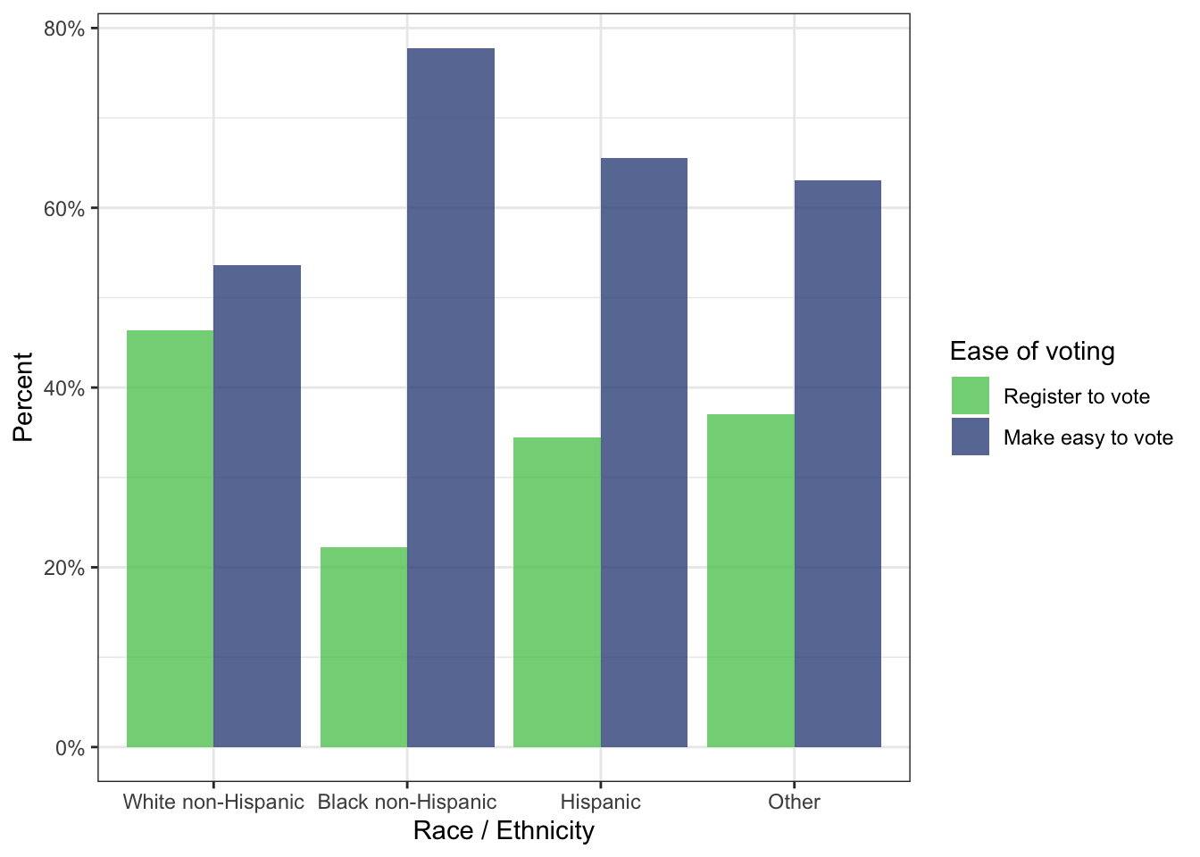
I had several difficulties by drawing this graph:
ease_vote has to be included by the fill argument. That seems not logical but together with position = dodge it make sense.dplyr::count())ggplot2::after_stat(). The solution was more trivial: Creating a new column with the calculated percentages and using geom_col() instead of geom_bar().Instead of the last line I could have used with the same result: ggplot2::geom_bar(position = "dodge", stat = "identity"). geom_bar() uses as standard option ggplot2::stat_count(). It is however possible to override the default value as was done in the book code. But it easier here to use geom_col() because it uses as default stat_identity() e.g., it leaves the data as is.
Two additional remarks:
R Code 5.14 : Visualizing opinions about ease of voting by race / ethnicity
vote_clean |>
    tidyr::drop_na(ease_vote) |>
    tidyr::drop_na(race) |>
    ggplot2::ggplot(
        ggplot2::aes(
            x = race,
            fill = ease_vote
        )
    ) +
    ggplot2::geom_bar(position = "dodge",
        ggplot2::aes(
            y = ggplot2::after_stat(count / base::sum(count))
        )) +
    ggplot2::scale_y_continuous(labels = scales::percent) +
    ggplot2::labs(
        x = "Race / Ethnicity",
        y = "Percent"
    ) +
    ggplot2::scale_fill_viridis_d(
        name = "Ease of voting",
        alpha = .8, # here alpha works!!
        begin = .25,
         end = .75,
        direction = -1,
        option = "viridis"
    )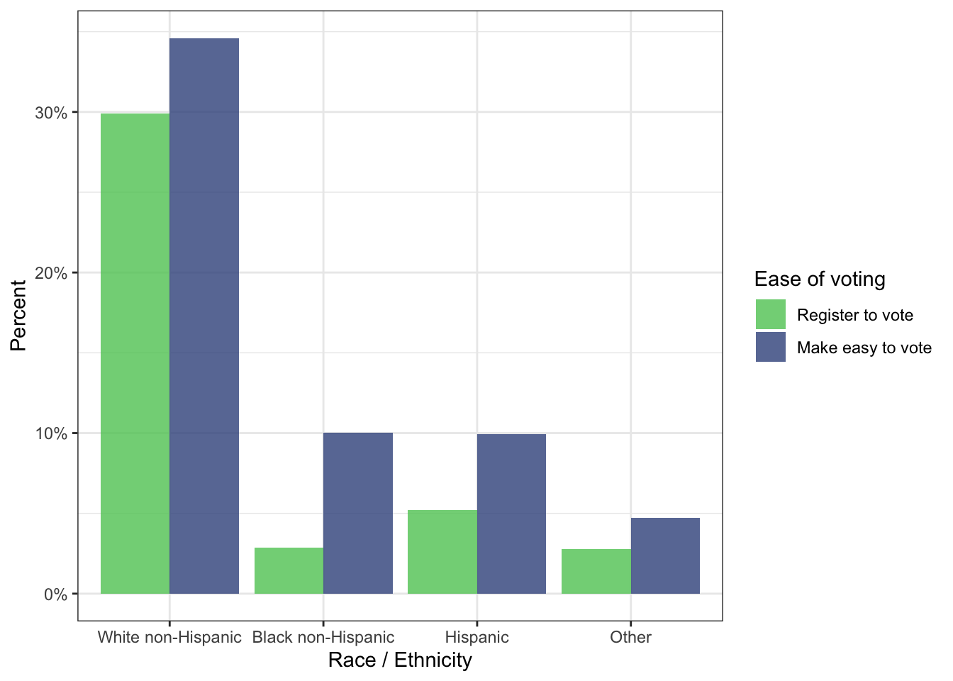
Here I have used geom_bar() with the after_stat() calculation. It turned out that the function computes the percentages of the different race categories for the two ease_vote values. This was not was I had intended.
I tried for several hours to use after_stat() with the same result as in R Code 5.13, but I didn’t succeed. I do not know if the reason is my missing knowledge (for instance to generate another structure of the data.frame) or if you can’t do that in general.
R Code 5.15 : Visualizing opinions about ease of voting by race / ethnicity
vote_clean |>
    tidyr::drop_na(ease_vote) |>
    tidyr::drop_na(race) |>
    dplyr::group_by(race, ease_vote) |>
    dplyr::count() |>
    dplyr::group_by(race) |>
    dplyr::mutate(perc = n / base::sum(n)) |>
    ggplot2::ggplot(
        ggplot2::aes(
            x = race,
            y = perc,
            fill = ease_vote)
    ) +
    ggplot2::geom_col(position = "dodge") +
    ggplot2::geom_label(
        ggplot2::aes(
            x = race,
            y = perc,
            label = paste0(round(100 * perc, 1),"%"),
            vjust = 1.5, hjust = -.035
        ),
        color = "white"
    ) +
    ggplot2::scale_y_continuous(labels = scales::percent) +
    ggplot2::labs(
        x = "Race / Ethnicity",
        y = "Percent"
    ) +
    ggplot2::scale_fill_viridis_d(
        name = "Ease of voting",
        alpha = .8, # here alpha works!!
        begin = .25,
         end = .75,
        direction = -1,
        option = "viridis"
    )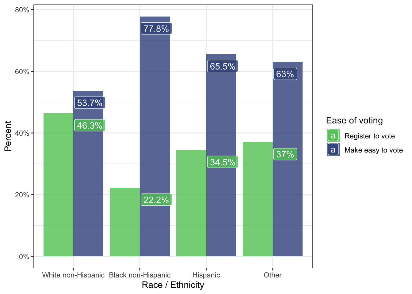
Here I have experimented with labels. It seems that with the argument position = dodge the labels can’t appear on each of the appropriate bars.
R Code 5.16 : Visualizing opinions about requirements of voting by race / ethnicity
p_require_vote <- vote_clean |>
    ## prepare data
    tidyr::drop_na(require_vote) |>
    tidyr::drop_na(race) |>
    dplyr::group_by(race, require_vote) |>
    dplyr::count() |>
    dplyr::group_by(race) |>
    dplyr::mutate(perc = n / base::sum(n)) |>

    ## draw graph
    ggplot2::ggplot(
        ggplot2::aes(
            x = race,
            y = perc,
            fill = require_vote)
    ) +
    ggplot2::geom_col(position = "dodge") +
    ggplot2::scale_y_continuous(labels = scales::percent) +
    ggplot2::labs(
        x = "Race / Ethnicity",
        y = "Percent"
    ) +
    ggplot2::scale_fill_viridis_d(
        name = "Requirements of voting",
        alpha = .8, # here alpha works!!
        begin = .25,
         end = .75,
        direction = -1,
        option = "viridis"
    )

p_require_vote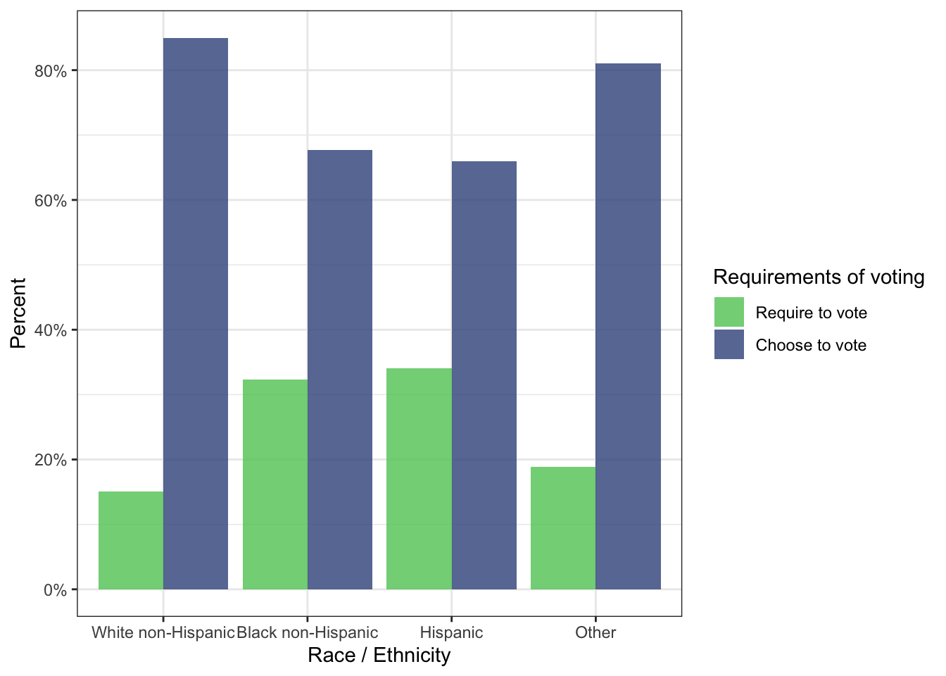
R Code 5.17 : Visualizing opinions about voting by race / ethnicity
p_ease <- p_ease_vote +
    ggplot2::labs(
        x = "",
        y = "Percent within group"
    ) +
    ggplot2::scale_fill_viridis_d(
        name = "Opinion on\nvoter registration",
        alpha = .8,
        begin = .25,
        end = .75,
        direction = -1,
        option = "viridis"
    ) +
    ggplot2::theme(axis.text.x = ggplot2::element_blank())

p_require <- p_require_vote +
    ggplot2::labs(y = "Percent within group") +
    ggplot2::scale_fill_viridis_d(
        name = "Opinion on\nvoting",
        alpha = .8,
        begin = .25,
        end = .75,
        direction = -1,
        option = "viridis"
    )

gridExtra::grid.arrange(p_ease, p_require, ncol = 1)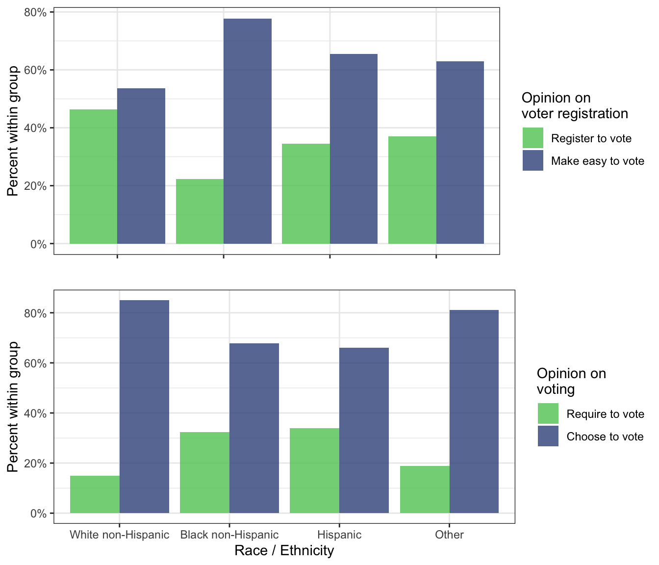
R Code 5.18 : Test how the colors used for the graph race by ease of voting look for printing in black & white
pal_data <- list(names = c("Normal", "desaturated"),
    color = list(scales::viridis_pal(
                                alpha = .8,
                                begin = .25,
                                 end = .75,
                                direction = -1,
                                option = "viridis")(2),
    colorspace::desaturate(scales::viridis_pal(
                                alpha = .8,
                                begin = .25,
                                end = .75,
                                direction = -1,
                                option = "viridis")(2)))
    )
list_plotter(pal_data$color, pal_data$names,
    "Colors and black & white of graph race by ease of voting")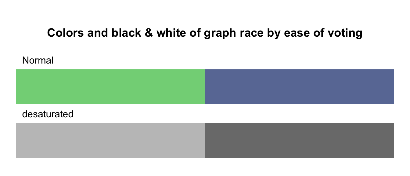
The chi-squared test is useful for testing to see if there may be a statistical relationship between two categorical variables. The chi-squared test is based on the observed values, and the values expected to occur if there were no relationship between the variables.
We will use the observed values from Listing / Output 5.2 and Listing / Output 5.3.
For each cell in the table, multiply the row total for that row by the column total for that column and divide by the overall total.
To prevent manually computing the values I have used CrossTable() from the {descr} package (see Section A.14 and StackOverflow).
\[ \text{Expected Values} = \frac{rowTotal \times columnTotal}{Total} \tag{5.1}\]
Example 5.3 : Show observed and expected values
R Code 5.19 : Ease of voting by race / ethnicity
vote_clean <- base::readRDS("data/chap05/vote_clean.rds")

vote_opinions <- vote_clean |>
    dplyr::select(race, ease_vote, require_vote) |>
    tidyr::drop_na()

ct_ease <- descr::CrossTable(
    x = vote_opinions$race,
    y = vote_opinions$ease_vote,
    dnn = c("Race", "Ease of voting"),
    prop.r = FALSE,
    prop.c = FALSE,
    prop.t = FALSE,
    prop.chisq = FALSE,
    expected = TRUE
    )
ct_ease
#> Cell Contents
#> |-------------------------|
#> | N |
#> | Expected N |
#> |-------------------------|
#>
#> ==================================================================
#> Ease of voting
#> Race Register to vote Make easy to vote Total
#> ------------------------------------------------------------------
#> White non-Hispanic 292 335 627
#> 255.5 371.5
#> ------------------------------------------------------------------
#> Black non-Hispanic 27 97 124
#> 50.5 73.5
#> ------------------------------------------------------------------
#> Hispanic 50 96 146
#> 59.5 86.5
#> ------------------------------------------------------------------
#> Other 25 45 70
#> 28.5 41.5
#> ------------------------------------------------------------------
#> Total 394 573 967
#> ==================================================================R Code 5.20 : Status of voting by race / ethnicity
ct_require <- descr::CrossTable(
        x = vote_opinions$race,
        y = vote_opinions$require_vote,
        dnn = c("Race", "Status of voting"),
        prop.r = FALSE,
        prop.c = FALSE,
        prop.t = FALSE,
        prop.chisq = FALSE,
        expected = TRUE
    )
ct_require
#> Cell Contents
#> |-------------------------|
#> | N |
#> | Expected N |
#> |-------------------------|
#>
#> ==============================================================
#> Status of voting
#> Race Require to vote Choose to vote Total
#> --------------------------------------------------------------
#> White non-Hispanic 95 532 627
#> 128.4 498.6
#> --------------------------------------------------------------
#> Black non-Hispanic 40 84 124
#> 25.4 98.6
#> --------------------------------------------------------------
#> Hispanic 50 96 146
#> 29.9 116.1
#> --------------------------------------------------------------
#> Other 13 57 70
#> 14.3 55.7
#> --------------------------------------------------------------
#> Total 198 769 967
#> ==============================================================The cell “Other” has similar observed and expected values, but the rest have bigger differences.
R Code 5.21 : Computing ease and require of voting using the {sjstats} package
## load vote_clean ##########
vote_clean <-  base::readRDS("data/chap05/vote_clean.rds")

vote_clean2 <- vote_clean |>
    dplyr::select(race, ease_vote, require_vote) |>
    tidyr::drop_na()

ease_vote_n <- vote_clean2 |>
    dplyr::select(race, ease_vote) |>
    dplyr::group_by(race, ease_vote) |>
    dplyr::summarize(n_ease = dplyr::n(),
                     .groups = "keep")

ease_expected  <-
    tibble::as_tibble(
        base::as.data.frame(
            sjstats::table_values(
                base::table(
                    vote_clean$race,
                    vote_clean$ease_vote)
                )$expected,
                .name_repair = "unique")) |>
    dplyr::arrange(Var1)

(
    ease_expected2 <- dplyr::bind_cols(
    ease_vote_n,
    exp_ease = ease_expected$Freq)
)

glue::glue(" ")
glue::glue("**********************************************************")
glue::glue(" ")

require_vote_n <- vote_clean2 |>
    dplyr::select(race, require_vote) |>
    dplyr::group_by(race, require_vote) |>
    dplyr::summarize(n_require = dplyr::n(),
                     .groups = "keep")

require_expected  <-
    tibble::as_tibble(
        base::as.data.frame(
            sjstats::table_values(
                base::table(
                    vote_clean$race,
                    vote_clean$require_vote)
                )$expected,
                .name_repair = "unique")) |>
    dplyr::arrange(Var1)

(
    require_expected2 <- dplyr::bind_cols(
    require_vote_n,
    exp_require = require_expected$Freq)
)
#> # A tibble: 8 × 4
#> # Groups: race, ease_vote [8]
#> race ease_vote n_ease exp_ease
#> <fct> <fct> <int> <dbl>
#> 1 White non-Hispanic Register to vote 292 257
#> 2 White non-Hispanic Make easy to vote 335 373
#> 3 Black non-Hispanic Register to vote 27 51
#> 4 Black non-Hispanic Make easy to vote 97 75
#> 5 Hispanic Register to vote 50 60
#> 6 Hispanic Make easy to vote 96 88
#> 7 Other Register to vote 25 30
#> 8 Other Make easy to vote 45 43
#>
#> **********************************************************
#>
#> # A tibble: 8 × 4
#> # Groups: race, require_vote [8]
#> race require_vote n_require exp_require
#> <fct> <fct> <int> <dbl>
#> 1 White non-Hispanic Require to vote 95 130
#> 2 White non-Hispanic Choose to vote 532 509
#> 3 Black non-Hispanic Require to vote 40 26
#> 4 Black non-Hispanic Choose to vote 84 101
#> 5 Hispanic Require to vote 50 30
#> 6 Hispanic Choose to vote 96 117
#> 7 Other Require to vote 13 15
#> 8 Other Choose to vote 57 59The sjstats::table_values() function has the advantage that it can be converted to a data.frame. We can therefore manipulate the data and — for example — combine expected data for different variables.
R Code 5.22 : : Combining ease and require of voting
#> # A tibble: 8 × 7
#> # Groups:   race, ease_vote [8]
#>   race              ease_vote n_ease exp_ease require_vote n_require exp_require
#>   <fct>             <fct>      <int>    <dbl> <fct>            <int>       <dbl>
#> 1 White non-Hispan… Register…    292      257 Require to …        95         130
#> 2 White non-Hispan… Make eas…    335      373 Choose to v…       532         509
#> 3 Black non-Hispan… Register…     27       51 Require to …        40          26
#> 4 Black non-Hispan… Make eas…     97       75 Choose to v…        84         101
#> 5 Hispanic          Register…     50       60 Require to …        50          30
#> 6 Hispanic          Make eas…     96       88 Choose to v…        96         117
#> 7 Other             Register…     25       30 Require to …        13          15
#> 8 Other             Make eas…     45       43 Choose to v…        57          59
Differences between observed values and expected indicates that there may be a relationship between the variables.
Bullet List
The differences between observed values and expected values can be combined into an overall statistic. But adding (resp. subtracting) does not work as the result is always 0. So we will again — like with the computation of the variance — square the difference.
To prevent huge differences when observed and expected values are very large, there is an additional step in the computation of \(\chi^2\): Divide the squared differences by the expected value of the appropriate cells.
\[ \chi^2 = \sum\frac{(observed - expected)^2}{expected} \tag{5.2}\]
R Code 5.23 : Compute chi-squared for race by ease of voting
vote_clean <- base::readRDS("data/chap05/vote_clean.rds")

stats::chisq.test(
    x = vote_clean$ease_vote,
    y = vote_clean$race
)
#>
#> Pearson's Chi-squared test
#>
#> data: vote_clean$ease_vote and vote_clean$race
#> X-squared = 28.952, df = 3, p-value = 2.293e-06In contrast to the binomial and normal distribution which both have two parameters (n and p, resp. \(\mu\) and \(\sigma\)), the chi-squared distribution has only one parameter: the degrees of freedom. The df can be used to find the population standard deviation for the distribution:
\[ \sqrt{2df} \tag{5.3}\]
Example 5.4 : Chi-square probability distributions with different degrees of freedom
R Code 5.24 : Four chi-square probability distributions with different degrees of freedom
# Define sequence of x-values
tib <- tibble::tibble(x = seq(0, 30, length.out = 600))

tib <- tib |>
# Compute density values
    dplyr::mutate(
        y1 = stats::dchisq(x, df = 1),
        y3 = stats::dchisq(x, df = 3),
        y5 = stats::dchisq(x, df = 5),
        y7 = stats::dchisq(x, df = 7)
    )
chi_sq1 <- tib |>
# Plot the Chi-square distribution: df = 1
    ggplot2::ggplot(ggplot2::aes(x = x, y = y1)) +
    ggplot2::geom_line(color = "blue") +
    ggplot2::labs(x = "x", y = "Density",
      title = paste("Chi-square with 1 degree of freedom"))

chi_sq3 <- tib |>
# Plot the Chi-square distribution: df = 3
    ggplot2::ggplot(ggplot2::aes(x = x, y = y3)) +
    ggplot2::geom_line(color = "blue") +
    ggplot2::labs(x = "x", y = "Density",
      title = paste("Chi-square with 3 degrees of freedom"))

chi_sq5 <- tib |>
# Plot the Chi-square distribution: df = 5
    ggplot2::ggplot(ggplot2::aes(x = x, y = y5)) +
    ggplot2::geom_line(color = "blue") +
    ggplot2::labs(x = "x", y = "Density",
      title = paste("Chi-square with 5 degrees of freedom"))

chi_sq7 <- tib |>
# Plot the Chi-square distribution: df = 7
    ggplot2::ggplot(ggplot2::aes(x = x, y = y7)) +
    ggplot2::geom_line(color = "blue") +
    ggplot2::labs(x = "x", y = "Density",
      title = paste("Chi-square with 7 degrees of freedom"))

gridExtra::grid.arrange(chi_sq1, chi_sq3, chi_sq5, chi_sq7, ncol = 2)
WATCH OUT! The graphs have different y scales!
This is the replication of Figure 5.7 from the book.
Note: The first impression — that all probability distributions have same height — is wrong! All four graphs have very different density scales!
We will see that all four distributions overlaid into one graphic will give a different impression.
R Code 5.25 : Four chi-square probability distributions with different degrees of freedom in one graph
# Define sequence of x-values
tib_chisq <- tibble::tibble(x = seq(0, 30, length.out = 600))

tib_chisq |>
# Compute density values
    dplyr::mutate(
        y1 = stats::dchisq(x, df = 1),
        y3 = stats::dchisq(x, df = 3),
        y5 = stats::dchisq(x, df = 5),
        y7 = stats::dchisq(x, df = 7)
    ) |>
    tidyr::pivot_longer(-1) |>

    ggplot2::ggplot(
        ggplot2::aes(x, value, color = name)) +
    ggplot2::geom_line(linewidth = 1) +
    ggplot2::ylim(0, .3) +
    ggplot2::labs(y = "Density") +
    ggplot2::scale_color_viridis_d(
        name = "Degrees\nof Freedom",
        labels = c("1", "3", "5", "7"),
        option = "plasma",
        end = .8
    )
See a more succinct example using a loop in How to Plot a Chi-Square Distribution in R (bprasad26 2023)
R Code 5.26 : Chi-square probability distributions with 3 degrees of freedom
ggplot2::ggplot() +
    ggplot2::xlim(0, 30) +
    ggplot2::stat_function(
        fun = dchisq,
        args = list(df = 3)
    )
Procedure 5.1 : Compute degrees of freedom (df) and population standard deviation of a chi-squared distribution
Example 5.5 : Compute degrees of freedom (df) and population standard deviation for the chi-squared distribution of race by ease_vote
I am following Procedure 5.1:
race: White non-Hispanic, Black non-Hispanic, Hispanic, Other. \(4 - 1 = 3\).ease_vote: Register to vote and Make easy to vote. \(2 - 1 = 1\).Multiply the resulting numbers together gives the degrees of freedom (df): \(3 \times 1 = 3\)
The population standard deviation is \(\sqrt{(2 \times df)}\) = \(\sqrt{(2 \times 3)}\) = 2.449.
The chi-squared distribution shown, which is the chi-squared probability density function (PDF), shows the probability of a value of chi-squared occurring when there is no relationship between the two variables contributing to the chi-squared.
Example 5.6 : Determine the probability using the chi-squared distribution
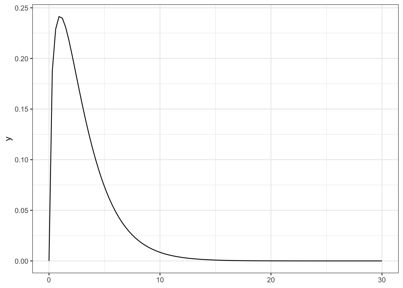
R Code 5.27 : Chi-squared probability distribution (df = 5)
## Define start of shade
x_shade = 10
y_shade = stats::dchisq(10, 5)


## Define sequence of x-values
tib <- tibble::tibble(x = seq(0, 30, length.out = 600)) |>
    # Compute density values
    dplyr::mutate(
        y = stats::dchisq(x, df = 5)
    )

## Subset data for shaded area
shade_10 <- tib |>
    dplyr::filter(x >= x_shade) |>
    ## Necessary as starting point for y = 0!
    tibble::add_row(x = 10, y = 0, .before = 1)


tib |>
    ## Plot the Chi-square distribution: df = 5
    ggplot2::ggplot(ggplot2::aes(x = x, y = y)) +
    ggplot2::geom_line() +

    ## Draw segment
    ggplot2::geom_segment(
        x = x_shade,
        y = 0,
        xend = x_shade,
        yend = y_shade
    ) +

    ## Shade curve
    ggplot2::geom_polygon(
        data = shade_10,
        fill = "lightblue",
        ggplot2::aes(x = x, y = y)
        ) +
    ggplot2::labs(x = "x", y = "Density",
      title = paste("Chi-square with 5 degree of freedom and shaded area starting with x = 10.0"))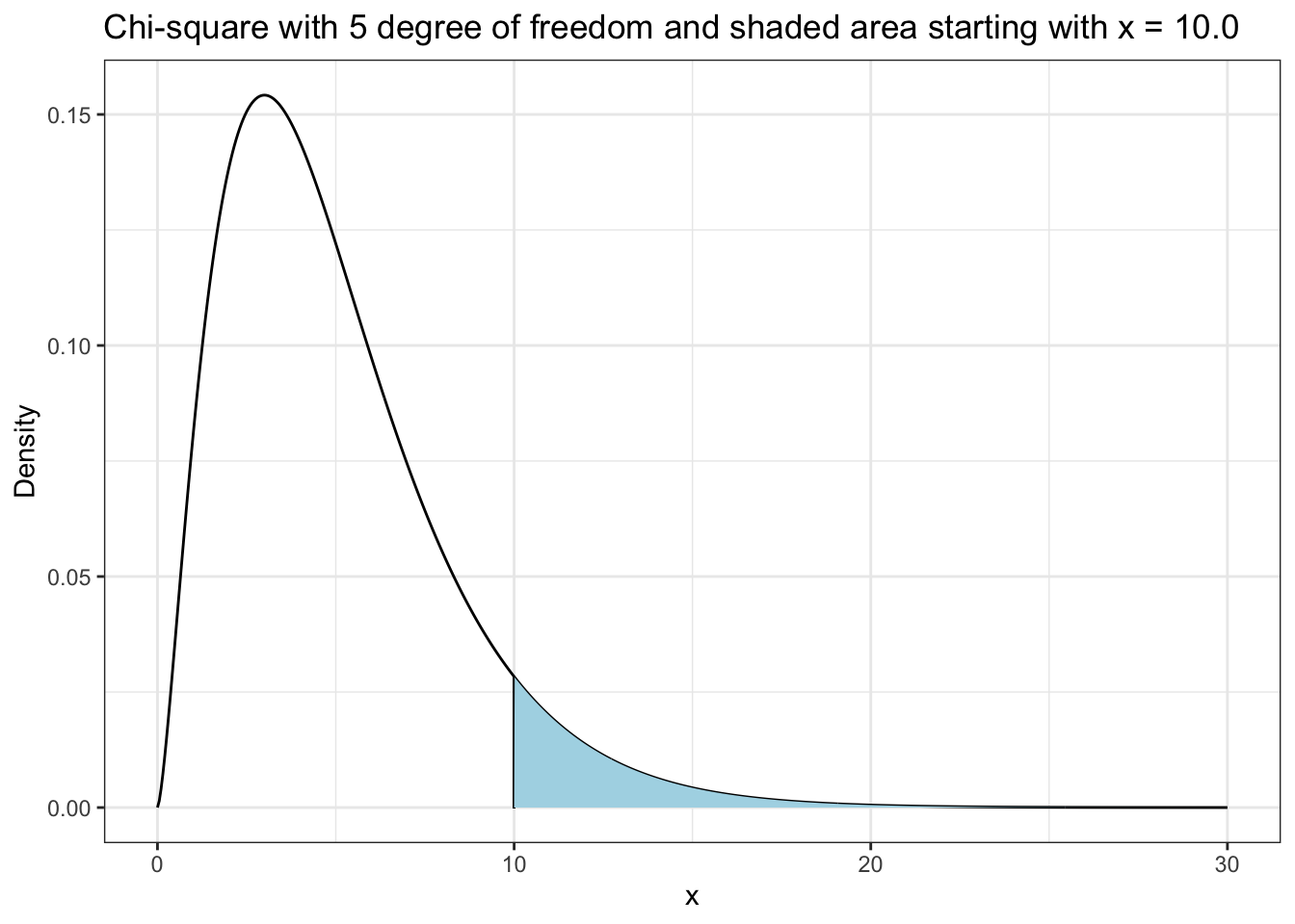
The probability that the differences between observed and expected values would result in a chi-squared of exactly 10 is — looking into the data — around 2.8%, e.g., very small.
It is more useful to know what the probability is of getting a chi-squared of 10 or higher. The probability of the chi-squared value being 10 or higher would be the area under the curve from 10 to the end of the distribution at the far right.
The probability of the chi-squared value being 10 or higher is about 15%. Even if this value is not very probable it is way above to be statistically significant (5%). The probability of the squared differences between observed and expected adding up to 10 or more is low when there is no relationship between the variables and result in a chi-squared value well inside the probability density function (PDF).
For instance: In our test case the \(\chi^2\)-value of 10.0 lies well inside the probability curve. The probability that this value can occur when there is no statistically relevant relationship is relatively high (15%). We can’t therefore reject the H0, because we do not have a statistically significant value of 5% or less. This can be seen clearly in the resulting graph of Listing / Output 5.6, created with the {sjPlot} package (see Section A.82).
R Code 5.28 : Chi-squared probability distribution (df = 5)
sjPlot::dist_chisq(chi2 = 10, deg.f = 5)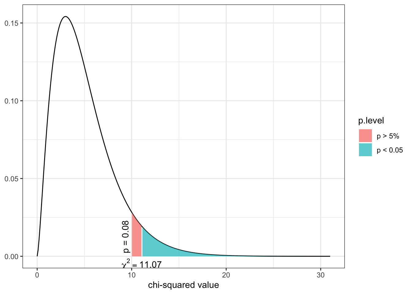
This graph uses the {sjPlot) package and is very easy to produce. It shows that the p-value for x = 10 is 0.08 (8%), e.g., higher as the standard value of 0.05 (5%). To be statistically significant, the \(\chi^2\) value would need to be equal or higher than 11.07.
{sjPlot}: Great package and easy to use in default mode, but you need time to learn the many configurations
Even if the standard version of the plot is easy to create, to adapt the graph is another issue. In the background {sjPlot} uses the {ggplot2} package, but you can’t specify changes by mixing (sjPlot) with {ggplot2} commands. I tried it and it produced two different plots. To customize plot appearance you have to learn the many arguments of of sjPlot:set_theme() and sjPlot::plot_grpfrq(). (See also Section A.82)
(I managed to change the theme in {sjPlot} by setting the default theme in {ggplot2} with ggplot2::theme_set(ggplot2::theme:bw()) as global option in the setup chunk.)
R Code 5.29 : Chi-squared probability distribution (df = 5)
nhstplot::plotchisqtest(chisq = 10, df = 5)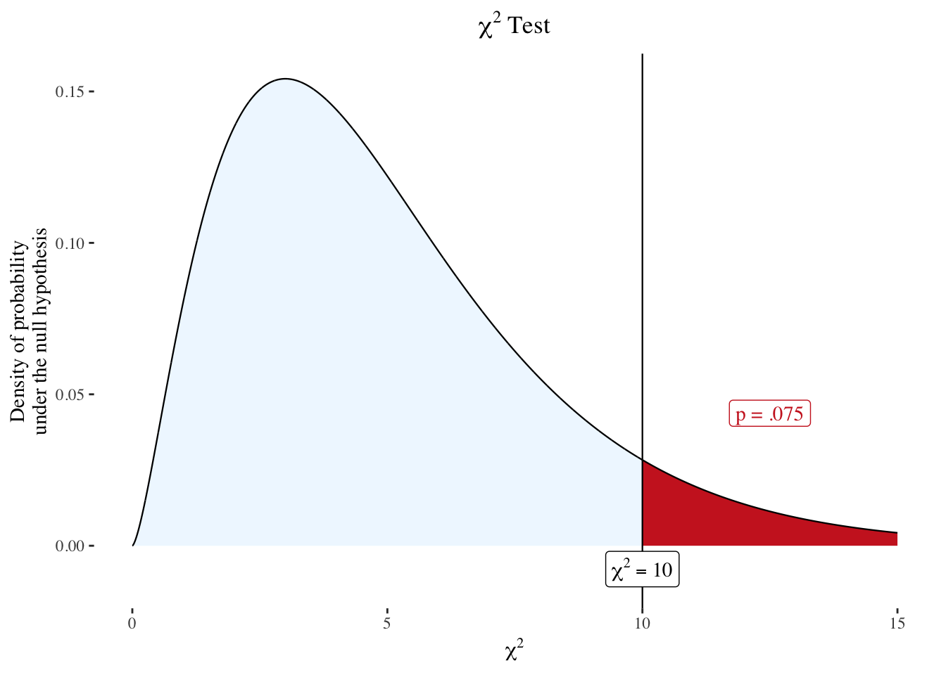
Working at 2024-04.26 on Chapter 10 I just learned of {nhstplot} as another package for illustrating graphically the most common Null Hypothesis Significance Testing (NHST) procedures (See Section A.54). This package is even easier to use than the {sjPlot) package and is more visually appealing.
Especially valuabe is that the axes are automatically scaled to present the relevant part and the overall shape of the probability density function. {nhstplot} is especially intended for education purposes, as it provides a helpful support to help explain the Null Hypothesis Significance Testing process, its use and/or shortcomings.
R Code 5.30 : Determine probability of ease of voting by race
(
    chisq_ease_vote_stats <- stats::chisq.test(ease_vote_table)
)

base::invisible(
    chisq_sjplot <- sjPlot::dist_chisq(
        chi2 = chisq_ease_vote_stats[["statistic"]][["X-squared"]],
        deg.f = chisq_ease_vote_stats[["parameter"]][["df"]]
        )
)
ease_vote by race#>
#> Pearson's Chi-squared test
#>
#> data: ease_vote_table
#> X-squared = 28.952, df = 3, p-value = 2.293e-06There is a statistically significant association between views on voting ease and race-ethnicity [\(\chi^2(3) = 28.95; p < .05\)].
Whenever possible, use the actual p-value rather than p < .05
In this case the p-value is so small that it wouldn’t look nice to provide the exact figure.
R Code 5.31 : Determine probability of ease of voting by race
(
    chisq_ease_vote_stats <- stats::chisq.test(ease_vote_table)
)


nhstplot::plotchisqtest(
    chisq = chisq_ease_vote_stats[["statistic"]][["X-squared"]],
    df = chisq_ease_vote_stats[["parameter"]][["df"]]
    )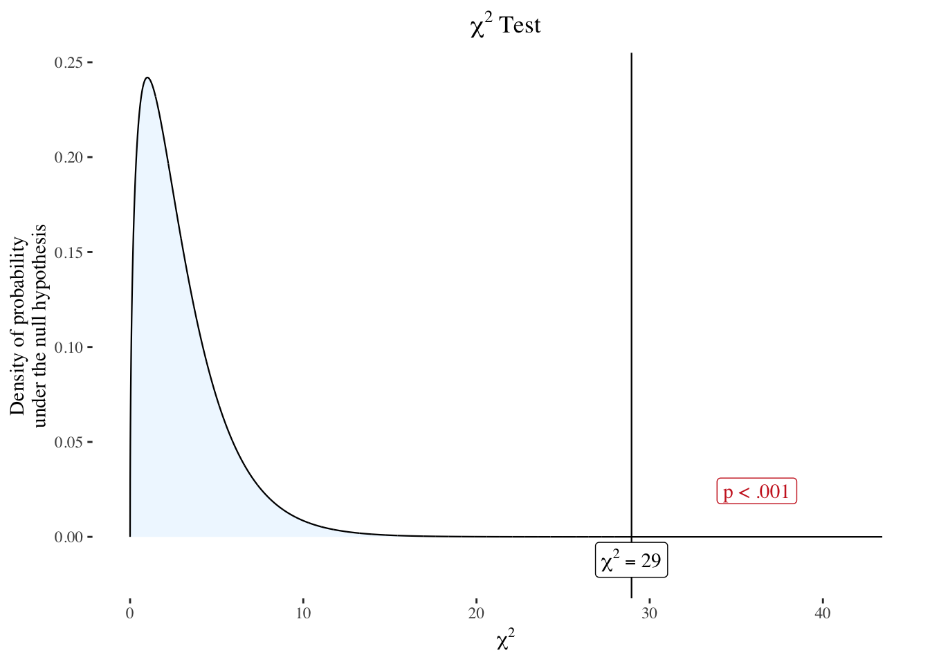
ease_vote by race#>
#> Pearson's Chi-squared test
#>
#> data: ease_vote_table
#> X-squared = 28.952, df = 3, p-value = 2.293e-06Procedure 5.2 : Null Hypothesis Significance Testing
WATCH OUT! Last step has to alternate options
In the book the above Procedure 5.2 has 5 options. But the last two steps (4 and 5) are contradictory alternatives. If one is true, the other does not apply. My Procedure 5.2 has therefore only 4 steps.
The null (H0) and alternate (HA) are written about the population and are tested using a sample from the population.
The second step is to use the test statistic. When examining a relationship between two categorical variables the appropriate test statistic is the chi-squared statistic, \(\chi^2\). You can see in the last line of Listing / Output 5.5 that \(\chi^2 = 28.952\).
The probability of seeing a chi-squared as big as 28.952 in our sample if there were no relationship in the population between opinion on voting ease and race-ethnicity group would be 0.000002293 or p < .05.
The probability that the null hypothesis, “People’s opinions on voter registration are the same across race-ethnicity groups,” is true in the population based on what we see in the sample is 0.000002293 or p < .05. This is a very small probability of being true and indicates that the null hypothesis is not likely to be true and should therefore be rejected.
We used the chi-squared test to test the null hypothesis that there was no relationship between opinions on voter registration and race/ethnicity group. We rejected the null hypothesis and concluded that there was a statistically significant association between views on voter registration and race-ethnicity [\(\chi^2(3) = 28.952; p < .05\)].
WATCH OUT! Chi-squared test and chi-squared goodness-of-fit test are not the same!
The chi-squared goodness-of-fit test is used for comparing the values of a single categorical variable to values from a hypothesized or population variable. The goodness-of-fit test is often used when trying to determine if a samples are a good representation of the population.
One limitation of the chi-squared independence test is that it determines whether or not there is a statistically significant relationship between two categorical variables but does not identify what makes the relationship significant. The name for this type of test is omnibus.
Standardized residuals (like z-scores can aid analysts in determining which of the observed frequencies are significantly larger or smaller than expected. The standardized residual is computed by subtracting the expected value in a cell from the observed value in a cell and dividing by the square root of the expected value.
\[ \text{Standardized residual} = \frac{observed - expected}{\sqrt{expected}} \tag{5.4}\]
The standardized residual is distributed like a z-score. Values of the standardized residuals that are higher than 1.96 or lower than –1.96 indicate that the observed value in that group is much higher or lower than the expected value. These are the groups that are contributing the most to a large chi-squared statistic and could be examined further and included in the interpretation.
WATCH OUT! Adjusted Standardized Residuals
There are also adjusted standardized residuals. To increase the confusion Alan Agresti (2018) calls these residuals “Standardized Pearson Residual”. To understand the difference between standardized and adjusted standardized residuals read see Standardized Residuals in Statistics: What are They? (Glen, n.d.b). Adjusted standardized residuals have higher values and are therefore not interpretable with the z-score values (e.g., looking for values greater or smaller than 2, res. 1.96 standard deviations). I will therefore stick with the (normal) standardized residuals.
\[ \begin{align*} & \text{Adjusted residual} = \\ & \frac{observed - expected}{\sqrt{expected \times (1-\text{row total proportion}) \times (1-\text{col total proportion}) )}} \end{align*} \tag{5.5}\]
The book recommends to get the standardized residuals with Descr::CrossTable(). But I have checked out that there are other possibilities as well.
Resource 5.3 Packages with functions to get standardized residuals of chi-squared tests
The following list collects these resources I have found together with the approximate average download data of the appropriate package. This figures will give you an idea about package use, but will not say anything about the quality of the package or the standardized residual function we are looking for.
stats::chisq.test()$residuals
descr::CrossTable(): It has arguments to show residuals, standardized residuals and adjusted standardized residualsjanitor::chisq.test(<tabyl>)$residuals
questionr::chisq.residuals()
rstatix::pearson_residuals(), rstatix::std_residuals()
There is also the possibility to use graphics::mosaicplot() with the option shade = TRUE to examine residuals visually for the source of differences (See (Greenwood 2022)).
R Code 5.32 : Number of daily downloads for packages with functions to display chi-squared residuals
#> # A tibble: 4 × 4
#>   package   average from       to
#>   <chr>       <dbl> <date>     <date>
#> 1 janitor      8105 2024-03-21 2024-03-27
#> 2 rstatix      5551 2024-03-21 2024-03-27
#> 3 questionr     682 2024-03-21 2024-03-27
#> 4 descr 469 2024-03-21 2024-03-27Example 5.7 : Compute standardized residuals with functions of different packages
R Code 5.33 : Compute standardized residuals with descr::CrossTable()
## load vote_clean ##########
vote_clean <-  base::readRDS("data/chap05/vote_clean.rds")

descr::CrossTable(
    x = ease_vote_table,
    expected = TRUE,
    prop.r = FALSE,
    prop.c = FALSE,
    prop.t = FALSE,
    prop.chisq = FALSE,
    chisq = TRUE,
    resid = TRUE,
    sresid = TRUE,
    asresid = TRUE
)
#> Cell Contents
#> |-------------------------|
#> | N |
#> | Expected N |
#> | Residual |
#> | Std Residual |
#> | Adj Std Resid |
#> |-------------------------|
#>
#> ==================================================================
#> Ease of voting
#> Race Register to vote Make easy to vote Total
#> ------------------------------------------------------------------
#> White non-Hispanic 292 338 630
#> 256.6 373.4
#> 35.357 -35.357
#> 2.207 -1.830
#> 4.811 -4.811
#> ------------------------------------------------------------------
#> Black non-Hispanic 28 98 126
#> 51.3 74.7
#> -23.329 23.329
#> -3.256 2.700
#> -4.532 4.532
#> ------------------------------------------------------------------
#> Hispanic 51 97 148
#> 60.3 87.7
#> -9.291 9.291
#> -1.197 0.992
#> -1.687 1.687
#> ------------------------------------------------------------------
#> Other 27 46 73
#> 29.7 43.3
#> -2.738 2.738
#> -0.502 0.416
#> -0.678 0.678
#> ------------------------------------------------------------------
#> Total 398 579 977
#> ==================================================================
#>
#> Statistics for All Table Factors
#>
#> Pearson's Chi-squared test
#> ------------------------------------------------------------
#> Chi^2 = 28.95154 d.f. = 3 p = 2.29e-06Here I have displayed the first and only time also the adjusted standardized residuals. As you can see they are much higher and do not obey the z-score distribution. I do not know how to interpret them. As far as I a understood they are only used for some software packages as e.g., SDA to highlight outstanding values. (See Watch-Out 5.1)
Bullet List
We used the chi-squared test to test the null hypothesis that there was no relationship between opinions on voter registration by race/ethnicity group. We rejected the null hypothesis and concluded that there was a statistically significant association between views on voter registration and race-ethnicity [\(\chi^2(3) = 28.95; p < .05\)]. Based on standardized residuals, the statistically significant chi-squared test result was driven by more White non-Hispanic participants and fewer Black non-Hispanic participants than expected believe that people should prove they want to vote by registering, and more Black non-Hispanic participants than expected believe that the voting process should be made easier.
R Code 5.34 : Compute standardized residuals with stats::chisq.test()
stats::chisq.test(ease_vote_table)$residuals
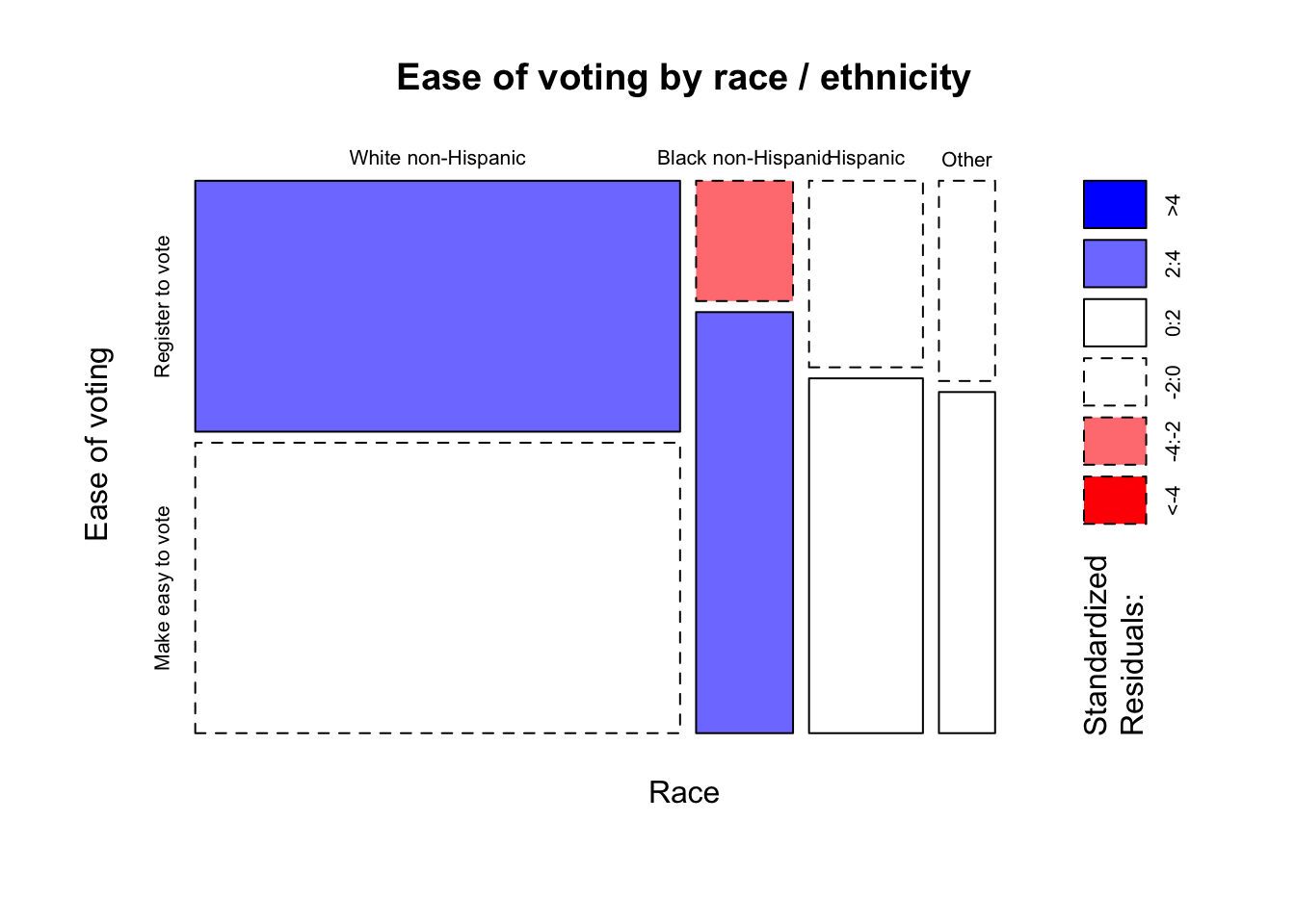
graphics::mosaicplot(
x = ease_vote_table,
shade = TRUE,
main = "Ease of voting by race / ethnicity"
)
#>                     Ease of voting
#> Race                 Register to vote Make easy to vote
#>   White non-Hispanic        2.2070569        -1.8298512
#>   Black non-Hispanic       -3.2561796         2.6996695
#>   Hispanic                 -1.1965274         0.9920302
#>   Other                    -0.5020807         0.4162707
I think that this result using base R tools is easier to understand and interpret as the presentation provided by descr::CrossTable(). Especially the graph highlights the important differences. Solid lines represent values higher whereas dashed lines point to proportion that are smaller than expected. And the color scale gives you immediate feedback about the size of difference.
R Code 5.35 : Compute standardized residuals with janitor::chisq.test()
janitor::chisq.test(ease_vote_table)$residuals#> Ease of voting
#> Race Register to vote Make easy to vote
#> White non-Hispanic 2.2070569 -1.8298512
#> Black non-Hispanic -3.2561796 2.6996695
#> Hispanic -1.1965274 0.9920302
#> Other -0.5020807 0.4162707Exactly the same result as with stats::chisq.test().
R Code 5.36 : Compute standardized residuals with questionr::chisq.residuals()
questionr::chisq.residuals(ease_vote_table)#> Ease of voting
#> Race Register to vote Make easy to vote
#> White non-Hispanic 2.21 -1.83
#> Black non-Hispanic -3.26 2.70
#> Hispanic -1.20 0.99
#> Other -0.50 0.42The only difference of this result is that the values are rounded. This is nice because for the interpretation we do not need the detailed values.
R Code 5.37 : Compute standardized residuals with rstatix::chisq_.residuals_test()
(chisq_ease_vote_rstatix <- rstatix::chisq_test(ease_vote_table))

rstatix::chisq_descriptives(chisq_ease_vote_rstatix)
#> # A tibble: 1 × 6
#> n statistic p df method p.signif
#> * <int> <dbl> <dbl> <int> <chr> <chr>
#> 1 977 29.0 0.00000229 3 Chi-square test ****
#> # A tibble: 8 × 9
#> Race Ease.of.voting observed prop row.prop col.prop expected resid
#> <fct> <fct> <int> <dbl> <dbl> <dbl> <dbl> <dbl>
#> 1 White non-Hi… Register to v… 292 0.299 0.463 0.734 257. 2.21
#> 2 Black non-Hi… Register to v… 28 0.0287 0.222 0.0704 51.3 -3.26
#> 3 Hispanic Register to v… 51 0.0522 0.345 0.128 60.3 -1.20
#> 4 Other Register to v… 27 0.0276 0.370 0.0678 29.7 -0.502
#> 5 White non-Hi… Make easy to … 338 0.346 0.537 0.584 373. -1.83
#> 6 Black non-Hi… Make easy to … 98 0.100 0.778 0.169 74.7 2.70
#> 7 Hispanic Make easy to … 97 0.0993 0.655 0.168 87.7 0.992
#> 8 Other Make easy to … 46 0.0471 0.630 0.0794 43.3 0.416
#> # ℹ 1 more variable: std.resid <dbl>The result with {rstatix} is very detailed. Using {rstatix} has the additioonal advantage that it is {tidyverse} compatible and you can use the pipe. The package includes many different tests and has with 7372 downloads from the RStudio CRAN mirror in one day (2024-11-11) a pretty big user group.
Which package should I use to show standardized residuals?
descr::CrossTable() is used in the book, but I can’t recommend it. The result cannot be transformed into a data.frame or tibble and it is therefore neither {tidyverse} compatible nor can you use the pipe.
A good solution is the combination of stats::chisq.test() and graphics::mosaicplot(). Especially the mosaic plot helps to figure out quickly which cells are important.
The best solution in my opinion is {rstatix}: Its results can be very detailed. {rstatix} is {tidyverse} compatible and you can use the pipe. The result with {rstatix} is very detailed. Using {rstatix} has the additional advantage that it is {tidyverse} compatible and you can use the pipe. The package includes many different tests and has with 7372 downloads from the RStudio CRAN mirror in one day (2024-11-11) a pretty big user group.) and can therefore used or other tasks as well. With 7372 downloads from the RStudio CRAN mirror in one day (2024-11-11) it has a pretty big user group.
Because of the wide range of tests and the big user basis I will apply {rstatix} as the predominant alternative whenever the result is the same with other packages.
Concerning out data about opinions about ease of voting we have two established two facts:
But we do not know the strength of this relationships. The strength of a relationship in statistics is referred to as effect size. For chi-squared, there are a few options, including the commonly used effect size statistic of Cramér’s V.
\[ V = \sqrt{\frac{\chi^2}{n(k-1)}} \tag{5.6}\]
\[ V = \sqrt{\frac{29.852}{977(2-1)}} = 0.17 \tag{5.7}\]
Assessment 5.1 : Interpretation of Cramér’s V
Cramér’s V is a measure of the strength of association between two nominal variables. It ranges from 0 to 1 where:
More detailed interpretation based on the degrees of freedom in How to Interpret Cramér’s V (with Examples) (Bobbitt, n.d.).
| Degrees of freedom | Small | Medium | Large |
|---|---|---|---|
| 1 | 0.10 | 0.30 | 0.50 |
| 2 | 0.07 | 0.21 | 0.35 |
| 3 | 0.06 | 0.17 | 0.29 |
| 4 | 0.05 | 0.15 | 0.25 |
| 5 | 0.04 | 0.13 | 0.22 |
Resource 5.4 Number of daily downloads for packages with functions to compute Cramér’s V
lsr::cramersV()
rcompanion::cramerV()
DescTools::CramerV()
sjstats::cramer()
rstatix::cramer_v()
collinear::cramber_v()
confintr::cramersv()
R Code 5.38 : Number of daily downloads for packages with functions to compute Cramèr’s V
#> # A tibble: 7 × 4
#>   package    average from       to
#>   <chr>        <dbl> <date>     <date>
#> 1 rstatix       5551 2024-03-21 2024-03-27
#> 2 DescTools     2099 2024-03-21 2024-03-27
#> 3 sjstats        841 2024-03-21 2024-03-27
#> 4 rcompanion     768 2024-03-21 2024-03-27
#> 5 lsr            452 2024-03-21 2024-03-27
#> 6 confintr       314 2024-03-21 2024-03-27
#> 7 collinear       10 2024-03-21 2024-03-27
I have checked only {lsr} and {rstatix} as I was happy with the result of the {rstatix} package.
Example 5.8 : Computing Cramér’s V
R Code 5.39 : Computing Cramér’s V with {lsr}
lsr::cramersV(ease_vote_table)#> [1] 0.1721427R Code 5.40 : Computing Cramér’s V with {rstatix}
rstatix::cramer_v(ease_vote_table)#> [1] 0.1721427The more conservative interpretation from the book sees the effect size between small and medium, corresponding to a relationship between weak to moderate Including the degrees of freedom we get the starting point for a moderate relationship. I will use the more conservative interpretation.
There is a statistically significant relationship between opinions on voter registration and race-ethnicity, and the relationship is weak to moderate. This is consistent with the frequencies, which are different from expected, but not by an enormous amount in most of the groups.
When both variables have just two categories then you should apply the Yates continuity correction. It subtracts an additional .5 from the difference between observed and expected in each group, or cell of the table, making the chi-squared test statistic value smaller, making it therefore harder to reach statistical significance.
The correction is necessary because the chi-squared distribution is not a perfect representation of the distribution of differences between observed and expected of a chi-squared test in the situation where both variables are binary. Normally functions apply the correction as default whenever two binary variables are tested but you can decide via an argument whether you want to apply the correction or not.
An exception is descr::CrossTable() which provides automatically both versions whenever you compute the test statistic for a 2 by 2 table. This is somewhat illogical because you would always need only the version with the correction for a 2 by 2 table (and not both) and sometimes you would also want to apply it when there are few observations in one or more of the cells.
Example 5.9 : Computing a chi-squared test statistic with the Yates continuity correction
R Code 5.41 : Chi-squared test for ease of voting and home ownership
## load vote_clean ##########
vote_clean <-  base::readRDS("data/chap05/vote_clean.rds")

descr::CrossTable(
    x = vote_clean$ease_vote,
    y = vote_clean$ownhome,
    expected = FALSE,
    prop.r = FALSE,
    prop.c = FALSE,
    prop.t = FALSE,
    prop.chisq = FALSE,
    chisq = TRUE,
    resid = FALSE,
    sresid = FALSE,
    asresid = FALSE
)
#> Cell Contents
#> |-------------------------|
#> | N |
#> |-------------------------|
#>
#> ==============================================
#> vote_clean$ownhome
#> vote_clean$ease_vote Owned Rented Total
#> ----------------------------------------------
#> Register to vote 287 112 399
#> ----------------------------------------------
#> Make easy to vote 375 208 583
#> ----------------------------------------------
#> Total 662 320 982
#> ==============================================
#>
#> Statistics for All Table Factors
#>
#> Pearson's Chi-squared test
#> ------------------------------------------------------------
#> Chi^2 = 6.240398 d.f. = 1 p = 0.0125
#>
#> Pearson's Chi-squared test with Yates' continuity correction
#> ------------------------------------------------------------
#> Chi^2 = 5.898905 d.f. = 1 p = 0.0152R Code 5.42 : Chi-squared test for ease of voting and home ownership with and without Yates continuity correction
vote_ownhome_chisq1 <- rstatix::chisq_test(
    vote_clean$ease_vote,
    vote_clean$ownhome,
    correct = FALSE
)

vote_ownhome_chisq2 <- rstatix::chisq_test(
    vote_clean$ease_vote,
    vote_clean$ownhome,
    correct = TRUE
)

vote_ownhome_chisq <-
    dplyr::bind_rows(
        vote_ownhome_chisq1,
        vote_ownhome_chisq2
        ) |>
    tibble::add_column(
        "Yates" = c("No", "Yes"),
        .before = "p.signif"
        )

vote_ownhome_chisq
#> # A tibble: 2 × 7
#> n statistic p df method Yates p.signif
#> <int> <dbl> <dbl> <int> <chr> <chr> <chr>
#> 1 1028 6.24 0.0125 1 Chi-square test No *
#> 2 1028 5.90 0.0152 1 Chi-square test Yes *To compare the differences I have computed the chi-squared test twice with and without Yates correction. Then I have combined the results and added a column with the label yes/no.
R Code 5.43 : Chi-squared test for ease of voting and home ownership
descr::CrossTable(
    x = vote_clean$ease_vote,
    y = vote_clean$ownhome,
    expected = TRUE,
    prop.r = FALSE,
    prop.c = FALSE,
    prop.t = FALSE,
    prop.chisq = FALSE,
    chisq = TRUE,
    resid = TRUE,
    sresid = TRUE,
    asresid = FALSE
)
#> Cell Contents
#> |-------------------------|
#> | N |
#> | Expected N |
#> | Residual |
#> | Std Residual |
#> |-------------------------|
#>
#> ===============================================
#> vote_clean$ownhome
#> vote_clean$ease_vote Owned Rented Total
#> -----------------------------------------------
#> Register to vote 287 112 399
#> 269 130
#> 18.02 -18.02
#> 1.099 -1.580
#> -----------------------------------------------
#> Make easy to vote 375 208 583
#> 393 190
#> -18.02 18.02
#> -0.909 1.307
#> -----------------------------------------------
#> Total 662 320 982
#> ===============================================
#>
#> Statistics for All Table Factors
#>
#> Pearson's Chi-squared test
#> ------------------------------------------------------------
#> Chi^2 = 6.240398 d.f. = 1 p = 0.0125
#>
#> Pearson's Chi-squared test with Yates' continuity correction
#> ------------------------------------------------------------
#> Chi^2 = 5.898905 d.f. = 1 p = 0.0152R Code 5.44 : Chi-squared test for ease of voting and home ownership with and without Yates continuity correction
vote_ownhome_chisq

glue::glue(" ")
glue::glue("#####################################################################")
glue::glue(" ")

rstatix::chisq_descriptives(vote_ownhome_chisq)
#> # A tibble: 2 × 7
#> n statistic p df method Yates p.signif
#> <int> <dbl> <dbl> <int> <chr> <chr> <chr>
#> 1 1028 6.24 0.0125 1 Chi-square test No *
#> 2 1028 5.90 0.0152 1 Chi-square test Yes *
#>
#> #####################################################################
#>
#> # A tibble: 4 × 9
#> x y observed prop row.prop col.prop expected resid std.resid
#> <fct> <fct> <int> <dbl> <dbl> <dbl> <dbl> <dbl> <dbl>
#> 1 Register to … Owned 287 0.292 0.719 0.434 269. 1.10 2.50
#> 2 Make easy to… Owned 375 0.382 0.643 0.566 393. -0.909 -2.50
#> 3 Register to … Rent… 112 0.114 0.281 0.35 130. -1.58 -2.50
#> 4 Make easy to… Rent… 208 0.212 0.357 0.65 190. 1.31 2.50To compare the differences I have computed the chi-squared test twice with and without Yates correction. Then I have combined the results and added a column with the label yes/no.
In all tabs of Example 5.9 you can see that with the Yates continuity correction the \(\chi^2\) value is smaller and results in a somewhat higher p-value. But that does not matter in this case: Both versions are statistically significant \(p < .05\).
Assessment 5.2 : What do the stars under the heading p-signif in the results of the chi-squared tests with {rstatix} mean?
| significance code |
p-value |
|---|---|
| *** | [0, 0.001] |
| ** | (0.001, 0.01] |
| * | (0.01, 0.05] |
| . | (0.05, 0.1] |
| (0.1, 1] |
R Code 5.45 : Computing the effect size with Cramér’s V
rstatix::cramer_v(
    vote_clean$ease_vote,
    vote_clean$ownhome,
    correct = TRUE
)
#> [1] 0.07750504The Yates continuity corrections also applies for the Cramér’s V effect size calculation. In this case the value of V falls into the weak or small effect size range.
Summary abbreviated
I have not followed the NHST procedure and the analysis of the relationship for ease of voting and home ownership. I understand and feel save about most of the content, therefore I focus only on material where I have difficulties or where I need more practice (as with the Yates continuity correction and Cramér’s V.
For 2 × 2 tables, the \(k – 1\) term in the denominator of the Cramér’s V formula is always 1, so this term is not needed in the calculation. The formula without this term is called the phi coefficient.
Formula 5.1 : Formula for phi coefficient \(\phi\)
\[ \phi = \sqrt{\frac{\chi^2}{n}} \tag{5.8}\]
n = sample size
Resource 5.5 Explaining the odds ratio
The explication in SwR is not easy to understand. So I have used other material a well:
Odds is usually defined in statistics as the probability an event will occur divided by the probability that it will not occur. In other words, it’s a ratio of successes (or wins) to losses (or failures). As an example, if a racehorse runs 100 races and wins 20 times, the odds of the horse winning a race is 20/80 = 1/4 = 0.25.
The odds definition is different to the somewhat similar definition of probability, which is the fraction of times an event occurs in a certain number of trials. In the horse example, the probability of a win is 20/100 = 0.2. (see (Glen, n.d.a))
Formula 5.2 : Formula for odds
\[ Odds = \frac{\text{Probability Event Occurs (p)}}{{\text{Probability Event Does Not Occur (1-p)}}} \tag{5.9}\]
Odds ratios with groups quantify the strength of the relationship between two conditions. They indicate how likely an outcome is to occur in one context relative to another.
Formula 5.3 : Formula for odds ratio
\[ \text{Odds Ratio} = \frac{\text{Odss of an Event (Condition A)}}{{\text{Odds of an Event (Condition B)}}} \tag{5.10}\]
The denominator (condition B) in the odds ratio formula is the baseline or control group. Consequently, the OR tells you how much more or less likely the numerator events (condition A) are likely to occur relative to the denominator events. If you have a treatment and control group, the treatment will be in the numerator while the control group is in the denominator of the formula (Frost 2022).
Taken the definition of odds and odds ratio together we get the formula:
Formula 5.4 : Formula for odds ration (2)
\[ \begin{align*} \text{Odds Ratio} = \frac{\text{Odds of an Event (Condition A)}}{{\text{Odds of an Event (Condition B)}}} = \\ \frac{\text{Odds of an Event (A)} / \text{Odds of an Non Event (A)}}{\text{Odds of an Event (B)} / \text{Odds of an Non Event (B)}} = \\ \frac{\text{Odds of an Event (A)} \times \text{Odds of an Non Event (B)}}{\text{Odds of Non Event (A)} \times \text{Odds of a Event (B)}} \end{align*} \tag{5.11}\]
The book explanation of the odds ratio uses with exposure and outcome two new concepts and is therefore more difficult to understand. Under this terminology is the odds ratio a measure of the likelihood of a particular outcome. The odds ratio is calculated as the ratio of the number of events that produce or are exposed to that outcome to the number of events that do not produce, resp. are not exposed to the outcome. The odds ratio measures the odds of some event or outcome occurring given a particular exposure compared to the odds of it happening without that exposure. Or more generally: The odds ratio tells us the ratio of the odds of an event occurring in a treatment group compared to the odds of an event occurring in a control group. (Still pretty difficult…)
In our case of voting opinion and housing status the odds ratio would measure the odds of people that think one should register to vote given owning a home, compared to the odds of people that think one should register to vote given not owning a home.
Formula 5.5 : Formula for odds ratio (3)
\[ OR = \frac{\text{exposed with outcome} / \text{unexposed with outcome}}{\text{exposed no outcome} / \text{unexposed no outcome}} \tag{5.12}\]
To fill in the correct values one has to conceptualize a 2x2 table:
R Code 5.46 : Odds ratio table
tibble::tribble(
  ~Exposure,      ~Cases,  ~Control,
  "Exposed",     "a",     "b",
  "Not Exposed", "c",     "d"
)
#> # A tibble: 2 × 3
#> Exposure Cases Control
#> <chr> <chr> <chr>
#> 1 Exposed a b
#> 2 Not Exposed c dThe columns “Cases” and “Control” are the Outcomes:
Formula 5.6 : Formula odds ratio (4)
\[ OR = \frac{a / c}{b / d} = \frac{a \times d}{b \times c} \tag{5.13}\]
Now let’s think what this general structure mean in our case with voting opinions (easy versus register) and housing status (owner or renter).
#>               Voting opinion
#> Housing status Register to vote Make easy to vote
#>         Owned               287               375
#>         Rented              112               208
Bullet List
Exposure and Outcome
Cells and their values
Assessment 5.3 : Interpretation of odds ratios using our example of voting opinion by housing status
General rule
Our example
\[ OR = \frac{a / c}{b / d} = \frac{287 / 112}{375 / 208} = \frac{2.5625}{1.802885} = 1.42 \tag{5.14}\]
The p-value for odds ratios has the same broad meaning as p-values for the chi-squared. But instead of being based on the area under the curve for the chi-squared distribution, it is based on the area under the curve for the log of the odds ratio, which is approximately normally distributed. The odds ratio can only be a positive number, and it results in a right-skewed distribution, which the log function can often transform to something close to normal.
Resource 5.6 Packages with odds ratio function
The book explains the manual calculation and recommends the {fmsb} package. I found via internet research some other packages with an odds ratio function: The following list is alphaetically sorted:
DescTools::OddsRatio()
epitools::oddsratio()
fmsb::oddsratio()
The packages {tern} and {BioProbability} feature also a odds ratio function. But I haven’t looked into these packages because they have less than 100 downloads daily form the RStudio CRAN Mirror server.
R Code 5.47 : Number of daily downloads for packages with an odds ratio function
pkgs = c("DescTools", "epitools", "fmsb", "tern", "BioProbability")
pkgs_dl(pkgs)#> # A tibble: 5 × 4
#> package average from to
#> <chr> <dbl> <date> <date>
#> 1 DescTools 3487 2024-11-05 2024-11-11
#> 2 fmsb 503 2024-11-05 2024-11-11
#> 3 epitools 427 2024-11-05 2024-11-11
#> 4 tern 46 2024-11-05 2024-11-11
#> 5 BioProbability 7 2024-11-05 2024-11-11Example 5.10 : Computing the odds ratio
R Code 5.48 : Odds ratio of ease of voting by home ownership computed manually
glue::glue("############### Table format used ################## ")
(
    vote_housing_table <- base::table(
        vote_clean$ownhome,
        vote_clean$ease_vote,
        dnn = c("Voting opinion", "Housing status")
    )
)
odds_ratio <-  round((287 / 112) / (375 / 208), 2)

glue::glue(" ")
glue::glue("###################################################")
glue::glue("Oddsratio: {odds_ratio}")
#> ############### Table format used ##################
#> Housing status
#> Voting opinion Register to vote Make easy to vote
#> Owned 287 375
#> Rented 112 208
#>
#> ###################################################
#> Oddsratio: 1.42The calculation uses the frequencies in the 2 × 2 table where the rows are the exposure and the columns are the outcome.
R Code 5.49 : Odds ratio of ease of voting by home ownership using fmsb::oddsratio()
#> Warning in N1 * N0 * M1 * M0: NAs produced by integer overflow#> ***************** Input counts manually ***********
#> Disease Nondisease Total
#> Exposed 287 375 662
#> Nonexposed 112 208 320
#> Total 399 583 982
#>
#> Odds ratio estimate and its significance probability
#>
#> data: 287 112 375 208
#> p-value = 0.01253
#> 95 percent confidence interval:
#> 1.078097 1.873847
#> sample estimates:
#> [1] 1.421333
#>
#>
#> *******************************************************
#> Disease Nondisease Total
#> Exposed 287 375 662
#> Nonexposed 112 208 320
#> Total 399 583 982
#>
#> Odds ratio estimate and its significance probability
#>
#> data: vote_housing_table
#> p-value = NA
#> 95 percent confidence interval:
#> 1.078097 1.873847
#> sample estimates:
#> [1] 1.421333Here I have replicated the code from the book. {fmsb} has a disadvantage: You have to specify the values manually, you can’t use a table object. It is said that the function will also work with a matrix but then I got a warning message:
Warning in N1 * N0 * M1 * M0: NAs produced by integer overflow
As a result of the produced NA’s the p-value is not computed. (But the calculated odds ratio is correct.)
So the best option is to stick with manually input. Besides of this inconvenience there is also a somewhat improper medical summary of the table (“Disease” / “Nondisease”).
R Code 5.50 : Odds ratio of ease of voting by home ownership using DescTools::OddsRatio()
DescTools::OddsRatio(
    x = vote_housing_table,
    conf.level = .95,
    method = "midp")
#> odds ratio lwr.ci upr.ci
#> 1.420209 1.078575 1.876316This is a very sparse output. In contrast to the two other packages it misses the table summary and the p-value.
R Code 5.51 : Odds ratio of ease of voting by home ownership using epitools::oddsratio()
epitools::oddsratio.midp(vote_housing_table,
                    correction = TRUE,
                    verbose = TRUE)
#> $x
#> Housing status
#> Voting opinion Register to vote Make easy to vote
#> Owned 287 375
#> Rented 112 208
#>
#> $data
#> Housing status
#> Voting opinion Register to vote Make easy to vote Total
#> Owned 287 375 662
#> Rented 112 208 320
#> Total 399 583 982
#>
#> $p.exposed
#> Housing status
#> Voting opinion Register to vote Make easy to vote Total
#> Owned 0.7192982 0.6432247 0.6741344
#> Rented 0.2807018 0.3567753 0.3258656
#> Total 1.0000000 1.0000000 1.0000000
#>
#> $p.outcome
#> Housing status
#> Voting opinion Register to vote Make easy to vote Total
#> Owned 0.4335347 0.5664653 1
#> Rented 0.3500000 0.6500000 1
#> Total 0.4063136 0.5936864 1
#>
#> $measure
#> odds ratio with 95% C.I.
#> Voting opinion estimate lower upper
#> Owned 1.000000 NA NA
#> Rented 1.420209 1.078575 1.876316
#>
#> $conf.level
#> [1] 0.95
#>
#> $p.value
#> two-sided
#> Voting opinion midp.exact fisher.exact chi.square
#> Owned NA NA NA
#> Rented 0.01235162 0.01268694 0.0151503
#>
#> $correction
#> [1] TRUE
#>
#> attr(,"method")
#> [1] "median-unbiased estimate & mid-p exact CI"This is the most detailed output. There exist also a less verbose version without
This more stringent version has the most important information and is in my opinion the best option for calculating the odds ratio.
{epitools} is my preferred method for the odds ratio calculation
Because of the somewhat inconvenient data input for the oddsratio() function of the {fmsb} package and the sparse output OddsRatio() function of the {DescTool} package I prefer the computation with {epitools} in its more stringent option (verbose = FALSE).
What is to do when one of the chi-squared assumption fails?
Use a different statistical test. Chi-squared is only appropriate for categorical variables.
The assumption of expected values of 5 or higher in at least 80% of groups is necessary because the sampling distribution for the chi-squared statistic only approximates the actual chi-squared distribution but does not capture it completely accurately. When a sample is large, the approximation is better and using the chi-squared distribution to determine statistical significance works well.
However, for very small samples, the approximation is not great, so a different method of computing the p-value is better. The method most commonly used is the Fisher’s exact test (stats::fisher.test(), rstatix::fisher_test(), janitor::fisher.test(), fmsb::pairwise.fisher.test()).
stats::mcnemar.test())nonpar::cochrans.q() the test is also availabe in other packages, that I used already for this book: DescTools::CochranQTest(), rstatix::cochran_qtest().| term | definition |
|---|---|
| Alternate Hypothesis | An alternate hypothesis (HA or sometimes written as H1) is a claim that there is a difference or relationship among things; the alternate hypothesis is paired with the null hypothesis that typcially states there is no relationship or no difference between things. (SwR, Glossary) |
| Chi-squared | Chi-squared is the test statistic following the chi-squared probability distribution; the chi-squared test statistic is used in inferential tests, including examining the association between two categorical variables and determining statistical significance for a logistic regression model. (SwR, Glossary) |
| Cochran’s Q-test | Cochran’s Q-test is an alternative to the chi-squared test of independence for when observations are not independent; for example, comparing groups before and after an intervention would fail the independent observations assumption (SwR, Glossary) |
| Cramér’s V | Cramér’s V is an effect size to determine the strength of the relationship between two categorical variables; often reported with the results of a chi-squared. (SwR, Glossary) |
| Degrees of Freedom | Degree of Freedom (df) is the number of pieces of information that are allowed to vary in computing a statistic before the remaining pieces of information are known; degrees of freedom are often used as parameters for distributions (e.g., chi-squared, F). (SwR, Glossary) |
| Effect Size | Effect size is a measure of the strength of a relationship; effect sizes are important in inferential statistics in order to determine and communicate whether a statistically significant result has practical importance. (SwR, Glossary) |
| Exposure | Exposure is a characteristic, behavior, or other factor that may be associated with an outcome. (SwR, Glossary) |
| Fisher’s exact test | Fisher’s exact test is an alternative to the chi-squared test for use with small samples. (SwR, Glossary) |
| McNemar’s test | McNemar’s test is an alternative to the chi-squared test of independence for when observations are not independent and both variables are binary; for example, McNemar’s test could be used to compare proportions in two groups before and after an intervention (SwR, Glossary) |
| NHST | Null Hypothesis Significance Testing (NHST) is a process for organizing inferential statistical tests. (SwR, Glossary) |
| Null Hypothesis | The null hypothesis (H0, or simply the Null) is a statement of no difference or no association that is used to guide statistical inference testing (SwR, Glossary) |
| Odds Ratio | Odds is usually defined in statistics as the probability an event will occur divided by the probability that it will not occur. An odds ratio (OR) is a measure of association between a certain property A and a second property B in a population. Specifically, it tells you how the presence or absence of property A has an effect on the presence or absence of property B. (<a href="https://www.statisticshowto.com/probability-and-statistics/probability-main-index/odds-ratio/">Statistics How To</a>). An odds ratio is a ratio of two ratios. They quantify the strength of the relationship between two conditions. They indicate how likely an outcome is to occur in one context relative to another. (<a href="https://statisticsbyjim.com/probability/odds-ratio/">Statistics by Jim</a>) |
| Omnibus | An omnibus is a statistical test that identifies that there is some relationship going on between variables, but not what that relationship is. (SwR, Glossary) |
| Outcome | Outcome is the variable being explained or predicted by a model; in linear and logistic regression, the outcome variable is on the left-hand side of the equal sign. (SwR, Glossary) |
| p-value | The p-value is the probability that the test statistic is at least as big as it is under the null hypothesis (SwR, Glossary) |
| Parameter | Unobserved variables are usually called Parameters. (SR2, Chap.2) A parameter is an unknown numerical characteristics of a population that must be estimated. (CDS). They are also numbers that govern statistical models ([stats.stackexchange](https://stats.stackexchange.com/a/255994/207389)). A parameter is also a number that is a defining characteristic of some population or a feature of a population. (SwR, Glossary) |
| Pew Research Center | The Pew Research Center (also simply known as Pew) is a nonpartisan American think tank based in Washington, D.C. It provides information on social issues, public opinion, and demographic trends shaping the United States and the world. It also conducts public opinion polling, demographic research, random sample survey research, and panel based surveys, media content analysis, and other empirical social science research. (<a href="https://en.wikipedia.org/wiki/Pew_Research_Center">Wikipedia</a>) |
| Phi coefficient | The phi coefficient is a meassure of effect size to determine the strength of the relationship between two binary variables; often reported with the results of a chi-squared test (SwR, Glossary) |
| Population | A population consists statistically of all the observations that fit some criterion; for example, all of the people currently living in the country of Bhutan or all of the people in the world currently eating strawberry ice cream. (SwR, Glossary) |
| Probability Density Function | A probability density function (PDF) tells us the probability that a random variable takes on a certain value. (<a href="https://www.statology.org/cdf-vs-pdf/">Statology</a>) The probability density function (PDF) for a given value of random variable X represents the density of probability (probability per unit random variable) within a particular range of that random variable X. Probability densities can take values larger than 1. ([StackExchange Mathematics](https://math.stackexchange.com/a/1464837/1215136)) We can use a continuous probability distribution to calculate the probability that a random variable lies within an interval of possible values. To do this, we use the continuous analogue of a sum, an integral. However, we recognise that calculating an integral is equivalent to calculating the area under a probability density curve. We use `p(value)` for probability densities and `P |
| Samples | Samples are subsets of observations from some population that is often analyzed to learn about the population sampled. (SwR, Glossary) |
| Standard Deviation | The standard deviation is a measure of the amount of variation or dispersion of a set of values. A low standard deviation indicates that the values tend to be close to the mean (also called the expected value) of the set, while a high standard deviation indicates that the values are spread out over a wider range. The standard deviation is the square root of its variance. A useful property of the standard deviation is that, unlike the variance, it is expressed in the same unit as the data. Standard deviation may be abbreviated SD, and is most commonly represented in mathematical texts and equations by the lower case Greek letter $\sigma$ (sigma), for the population standard deviation, or the Latin letter $s$ for the sample standard deviation. ([Wikipedia](https://en.wikipedia.org/wiki/Standard_deviation)) |
| Standardized Residuals | Standardized residuals are the standardized differences between observed and expected values in a chi-squared analysis; a large standardized residual indicates that the observed and expected values were very different. (SwR, Glossary) |
| SwR | SwR is my abbreviation of: Harris, J. K. (2020). Statistics With R: Solving Problems Using Real-World Data (Illustrated Edition). SAGE Publications, Inc. |
| Yates continuity correction | Yates continuity correction is a correction for chi-squared that subtracts .5 from the difference between observed and expected in each cell, making the chi-squared value smaller and statistical significance harder to reach; it is often used when there are few observations in one or more of the cells. This correction is also used when both variables have just two categories because the chi-squared distribution is not a perfect representation of the distribution of differences between observed and expected of a chi-squared in the situation where both variables are binary. (SwR, Glossary and Chap. 5) |
| Z-score | A z-score (also called a standard score) gives you an idea of how far from the mean a data point is. But more technically it’s a measure of how many standard deviations below or above the population mean a raw score is. (<a href="https://www.statisticshowto.com/probability-and-statistics/z-score/#Whatisazscore">StatisticsHowTo</a>) |
Session Info
sessioninfo::session_info()#> ─ Session info ───────────────────────────────────────────────────────────────
#> setting value
#> version R version 4.4.2 (2024-10-31)
#> os macOS Sequoia 15.1
#> system x86_64, darwin20
#> ui X11
#> language (EN)
#> collate en_US.UTF-8
#> ctype en_US.UTF-8
#> tz Europe/Vienna
#> date 2024-11-13
#> pandoc 3.5 @ /usr/local/bin/ (via rmarkdown)
#>
#> ─ Packages ───────────────────────────────────────────────────────────────────
#> package * version date (UTC) lib source
#> abind 1.4-8 2024-09-12 [2] CRAN (R 4.4.1)
#> backports 1.5.0 2024-05-23 [2] CRAN (R 4.4.0)
#> base64enc 0.1-3 2015-07-28 [2] CRAN (R 4.4.0)
#> boot 1.3-31 2024-08-28 [2] CRAN (R 4.4.2)
#> broom 1.0.7 2024-09-26 [2] CRAN (R 4.4.1)
#> car 3.1-3 2024-09-27 [2] CRAN (R 4.4.1)
#> carData 3.0-5 2022-01-06 [2] CRAN (R 4.4.0)
#> cellranger 1.1.0 2016-07-27 [2] CRAN (R 4.4.0)
#> class 7.3-22 2023-05-03 [2] CRAN (R 4.4.2)
#> cli 3.6.3 2024-06-21 [2] CRAN (R 4.4.1)
#> codetools 0.2-20 2024-03-31 [2] CRAN (R 4.4.2)
#> colorspace 2.1-1 2024-07-26 [2] CRAN (R 4.4.0)
#> commonmark 1.9.2 2024-10-04 [2] CRAN (R 4.4.1)
#> cranlogs 2.1.1 2019-04-29 [2] CRAN (R 4.4.0)
#> crayon 1.5.3 2024-06-20 [2] CRAN (R 4.4.0)
#> curl 6.0.0 2024-11-05 [2] CRAN (R 4.4.1)
#> data.table 1.16.2 2024-10-10 [2] CRAN (R 4.4.1)
#> datawizard 0.13.0 2024-10-05 [2] CRAN (R 4.4.1)
#> descr 1.1.8 2023-11-27 [2] CRAN (R 4.4.0)
#> DescTools 0.99.58 2024-11-08 [2] CRAN (R 4.4.1)
#> digest 0.6.37 2024-08-19 [2] CRAN (R 4.4.1)
#> dplyr 1.1.4 2023-11-17 [2] CRAN (R 4.4.0)
#> e1071 1.7-16 2024-09-16 [2] CRAN (R 4.4.1)
#> epitools 0.5-10.1 2020-03-22 [2] CRAN (R 4.4.0)
#> evaluate 1.0.1 2024-10-10 [2] CRAN (R 4.4.1)
#> Exact 3.3 2024-07-21 [2] CRAN (R 4.4.0)
#> expm 1.0-0 2024-08-19 [2] CRAN (R 4.4.1)
#> fansi 1.0.6 2023-12-08 [2] CRAN (R 4.4.0)
#> farver 2.1.2 2024-05-13 [2] CRAN (R 4.4.0)
#> fastmap 1.2.0 2024-05-15 [2] CRAN (R 4.4.0)
#> fmsb 0.7.6 2024-01-19 [2] CRAN (R 4.4.0)
#> forcats 1.0.0 2023-01-29 [2] CRAN (R 4.4.0)
#> Formula 1.2-5 2023-02-24 [2] CRAN (R 4.4.0)
#> generics 0.1.3 2022-07-05 [2] CRAN (R 4.4.0)
#> ggeffects 1.7.2 2024-10-13 [2] CRAN (R 4.4.1)
#> ggplot2 3.5.1 2024-04-23 [2] CRAN (R 4.4.0)
#> gld 2.6.6 2022-10-23 [2] CRAN (R 4.4.0)
#> glossary * 1.0.0.9003 2024-08-05 [2] Github (debruine/glossary@05e4a61)
#> glue 1.8.0 2024-09-30 [2] CRAN (R 4.4.1)
#> gridExtra 2.3 2017-09-09 [2] CRAN (R 4.4.0)
#> gtable 0.3.6 2024-10-25 [2] CRAN (R 4.4.1)
#> haven 2.5.4 2023-11-30 [2] CRAN (R 4.4.0)
#> here 1.0.1 2020-12-13 [2] CRAN (R 4.4.0)
#> highr 0.11 2024-05-26 [2] CRAN (R 4.4.0)
#> hms 1.1.3 2023-03-21 [2] CRAN (R 4.4.0)
#> htmltools 0.5.8.1 2024-04-04 [2] CRAN (R 4.4.0)
#> htmlwidgets 1.6.4 2023-12-06 [2] CRAN (R 4.4.0)
#> httpuv 1.6.15 2024-03-26 [2] CRAN (R 4.4.0)
#> httr 1.4.7 2023-08-15 [2] CRAN (R 4.4.0)
#> insight 0.20.5 2024-10-02 [2] CRAN (R 4.4.1)
#> janitor 2.2.0 2023-02-02 [2] CRAN (R 4.4.0)
#> jsonlite 1.8.9 2024-09-20 [2] CRAN (R 4.4.1)
#> kableExtra 1.4.0 2024-01-24 [2] CRAN (R 4.4.0)
#> knitr 1.49 2024-11-08 [2] CRAN (R 4.4.1)
#> labeling 0.4.3 2023-08-29 [2] CRAN (R 4.4.0)
#> labelled 2.13.0 2024-04-23 [2] CRAN (R 4.4.0)
#> later 1.3.2 2023-12-06 [2] CRAN (R 4.4.0)
#> lattice 0.22-6 2024-03-20 [2] CRAN (R 4.4.2)
#> lifecycle 1.0.4 2023-11-07 [2] CRAN (R 4.4.0)
#> lmom 3.2 2024-09-30 [2] CRAN (R 4.4.1)
#> lsr 0.5.2 2021-12-01 [2] CRAN (R 4.4.0)
#> lubridate 1.9.3 2023-09-27 [2] CRAN (R 4.4.0)
#> magrittr 2.0.3 2022-03-30 [2] CRAN (R 4.4.0)
#> markdown 1.13 2024-06-04 [2] CRAN (R 4.4.0)
#> MASS 7.3-61 2024-06-13 [2] CRAN (R 4.4.2)
#> Matrix 1.7-1 2024-10-18 [2] CRAN (R 4.4.2)
#> mime 0.12 2021-09-28 [2] CRAN (R 4.4.0)
#> miniUI 0.1.1.1 2018-05-18 [2] CRAN (R 4.4.0)
#> munsell 0.5.1 2024-04-01 [2] CRAN (R 4.4.0)
#> mvtnorm 1.3-2 2024-11-04 [2] CRAN (R 4.4.1)
#> naniar 1.1.0 2024-03-05 [2] CRAN (R 4.4.0)
#> nhstplot 1.3.0 2024-03-01 [2] CRAN (R 4.4.0)
#> performance 0.12.4 2024-10-18 [2] CRAN (R 4.4.1)
#> pillar 1.9.0 2023-03-22 [2] CRAN (R 4.4.0)
#> pkgconfig 2.0.3 2019-09-22 [2] CRAN (R 4.4.0)
#> promises 1.3.0 2024-04-05 [2] CRAN (R 4.4.0)
#> proxy 0.4-27 2022-06-09 [2] CRAN (R 4.4.0)
#> purrr 1.0.2 2023-08-10 [2] CRAN (R 4.4.0)
#> questionr 0.7.8 2023-01-31 [2] CRAN (R 4.4.0)
#> R6 2.5.1 2021-08-19 [2] CRAN (R 4.4.0)
#> Rcpp 1.0.13-1 2024-11-02 [1] CRAN (R 4.4.1)
#> readxl 1.4.3 2023-07-06 [2] CRAN (R 4.4.0)
#> repr 1.1.7 2024-03-22 [2] CRAN (R 4.4.0)
#> rlang 1.1.4 2024-06-04 [2] CRAN (R 4.4.0)
#> rmarkdown 2.29 2024-11-04 [2] CRAN (R 4.4.1)
#> rootSolve 1.8.2.4 2023-09-21 [2] CRAN (R 4.4.0)
#> rprojroot 2.0.4 2023-11-05 [2] CRAN (R 4.4.0)
#> rstatix 0.7.2 2023-02-01 [2] CRAN (R 4.4.0)
#> rstudioapi 0.17.1 2024-10-22 [2] CRAN (R 4.4.1)
#> rversions 2.1.2 2022-08-31 [2] CRAN (R 4.4.0)
#> scales 1.3.0 2023-11-28 [2] CRAN (R 4.4.0)
#> sessioninfo 1.2.2 2021-12-06 [2] CRAN (R 4.4.0)
#> shiny 1.9.1 2024-08-01 [2] CRAN (R 4.4.0)
#> sjlabelled 1.2.0 2022-04-10 [2] CRAN (R 4.4.0)
#> sjmisc 2.8.10 2024-05-13 [2] CRAN (R 4.4.0)
#> sjPlot 2.8.16 2024-05-13 [2] CRAN (R 4.4.0)
#> sjstats 0.19.0 2024-05-14 [2] CRAN (R 4.4.0)
#> skimr 2.1.5 2022-12-23 [2] CRAN (R 4.4.0)
#> snakecase 0.11.1 2023-08-27 [2] CRAN (R 4.4.0)
#> stringi 1.8.4 2024-05-06 [2] CRAN (R 4.4.0)
#> stringr 1.5.1 2023-11-14 [2] CRAN (R 4.4.0)
#> svglite 2.1.3 2023-12-08 [2] CRAN (R 4.4.0)
#> systemfonts 1.1.0 2024-05-15 [2] CRAN (R 4.4.0)
#> tibble 3.2.1 2023-03-20 [2] CRAN (R 4.4.0)
#> tidyr 1.3.1 2024-01-24 [2] CRAN (R 4.4.0)
#> tidyselect 1.2.1 2024-03-11 [2] CRAN (R 4.4.0)
#> timechange 0.3.0 2024-01-18 [2] CRAN (R 4.4.0)
#> utf8 1.2.4 2023-10-22 [2] CRAN (R 4.4.0)
#> vctrs 0.6.5 2023-12-01 [2] CRAN (R 4.4.0)
#> viridisLite 0.4.2 2023-05-02 [2] CRAN (R 4.4.0)
#> visdat 0.6.0 2023-02-02 [2] CRAN (R 4.4.0)
#> withr 3.0.2 2024-10-28 [2] CRAN (R 4.4.1)
#> xfun 0.49 2024-10-31 [2] CRAN (R 4.4.1)
#> xml2 1.3.6 2023-12-04 [2] CRAN (R 4.4.0)
#> xtable 1.8-4 2019-04-21 [2] CRAN (R 4.4.0)
#> yaml 2.3.10 2024-07-26 [2] CRAN (R 4.4.0)
#>
#> [1] /Library/Frameworks/R.framework/Versions/4.4-x86_64/library
#> [2] /Library/Frameworks/R.framework/Versions/4.4-x86_64/Resources/library
#>
#> ──────────────────────────────────────────────────────────────────────────────Not Daniel Navarro as mentioned in the book. Danielle has changed her gender.↩︎