Code
#>     grass               age
#>  Length:2867        Length:2867
#>  Class :character   Class :character
#> Mode :character Mode :characterObjectives for chapter 01
SwR Achievements
I will skip the crossed out learning objectives in parenthesis as I know already these procedures. However I will modify and elaborate some of these achievements as mentioned in the parentheses.
I will add other objectives that resulted from questions that arose during reading the book.
Questions that resulted to additional objectives
SwR explains writing script files, but I am using Literate Programming with Quarto. This has the consequence that in addition to short comments inside code cells I have the possibility to write extensively in the other parts of the file about approach, code, results etc.
A practical advice for scripts is to include a prolog. Possible prolog sections:
Most of these information are naturally occurring in the writing process of Quarto books.
Resource 1.1 : Literate Statistical Programming
I am used to apply the tidyverse style guide. It requires to use underlines (“snake_code”) as separators in object names. (In contrast to “camelCase” code style). But reading the book I thought it might be a good idea to use special additional styles for certain specific objects.
k_... I had already experienced that didn’t know from which package a function was. Only to learn after looking around for minutes that it was a function I wrote myself!df_ for data.frame and dt_ for tibble. I might also use a suffix to refer to the status e.g., _raw (raw data), _clean (cleaned data), _v2 (version number).chap02_. And maybe also — as in naming data frames — the status as suffix.R has many possibilities to import data from other statistical packages.
I will not go into the import details of all the different packages here, because my focus is on the General Social Survey (GSS) data.
“While the GSS data can be read into R directly from the GSS website, Kiara had experienced this and knew that it could be frustrating.” (Harris, 2020) (pdf)
The author therefore offers for this chapter a .csv file with the data. In later chapters learner can choose to use the provided files from the SAGE webpage. Even if these data files are not yet cleaned, it is a kind of cheating, because it bypasses downloading data from the original source.
The pb_create_folder() function in the following code chunk checks if the folder already exists. If this is the case it leaves it untouched, otherwise it creates the folder at the desired path. The code for my private functions are in the file helper.R inside the R folder at root level of this working directory.
Example 1.1 : Read data from a .csv file into R
R Code 1.1 : Read .csv file and show data summary
#> grass age
#> Length:2867 Length:2867
#> Class :character Class :character
#> Mode :character Mode :characterbase::summary()
Some comments
base::read.csv() in the book I used with readr::read_csv() a function from the {tidyverse} package collection.show_col_types = FALSE argument to prevent a message about the column specification.The output of base::summary is in this case not very informative. Looking around for appropriate reporting function I developed with my_glance_data() my private command. (See Listing / Output 1.2 in next tab.)
R Code 1.2 Look at data with my private function my_glance_data()
#> # A tibble: 10 × 3
#>      obs age   grass
#>    <int> <chr> <chr>
#>  1     1 47    IAP
#>  2   172 27    LEGAL
#>  3   562 70    NOT LEGAL
#>  4   898 60    NOT LEGAL
#>  5  1019 30    LEGAL
#>  6  1176 80    NOT LEGAL
#>  7  1505 53    IAP
#>  8  1911 54    NOT LEGAL
#>  9  2622 62    IAP
#> 10 2867 72 NOT LEGALI developed a private function my_glance_data() to provide a first impression about the data. The function prints the first and last row of the dataset, so you know implicitly how many rows the dataset has. Between the first and last row the function adds randomly N other rows (default is 8). Additionally it provides the row number of the data in a separate column. (The column header obs stands for “observation”.) For reproducibility purposes you can also add a number for the set.seed() command.
The idea of my_glance_data() is to get a first impression of the dataset. Other printing methods show only the first (or last) rows of the dataset. This could be misleading, giving a wrong impression about typical data.
Maybe you are interested to use my_glance_data() yourself? It isn’t available through a package, but you can copy the source code from the next R chunk.
I have saved the function in a .qmd file one level higher as this book (and all my other R projects). With {{< include "../_common.qmd" >}} I have the code integrated in this book. (For the include shortcode see the section Includes of the Quarto documentation.)
### function my_glance_data ##############
my_glance_data <- function(df, N = 8, seed = 42){
    df_temp <- first_and_last_row(df)

    set.seed(seed)
    df |>
    dplyr::mutate(obs = dplyr::row_number()) |>
    dplyr::relocate(obs) |>
    dplyr::slice_sample(n = N) |>
    dplyr::bind_rows(df_temp) |>
    dplyr::arrange(obs)
}

first_and_last_row <-  function(df) {
    df |>
    dplyr::mutate(obs = dplyr::row_number()) |>
    dplyr::filter(dplyr::row_number() %in% base::c(1, dplyr::n()))
}glance_date()
After we saved the data we need to do some data wrangling. To replicate the data structure for the book Figure 1.2 we need to:
age and grass to work withgrass into factorgrass labelsage from double to numericage into appropriate age intervals and label them accordingly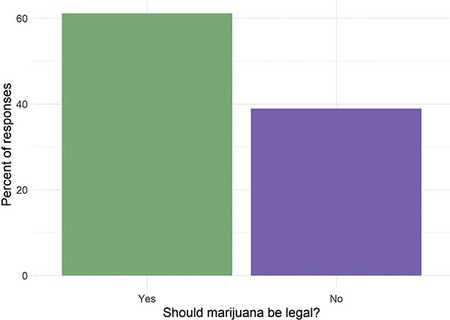
Example 1.2 : Replicate data structure for bar charts
R Code 1.3 : Replicate data structure for Figures 1.1 and 1.2 (Book)
gss_2016 <- readr::read_csv(
    file = "data/chap01/legal_weed_age_GSS2016_ch1.csv",
    show_col_types = FALSE)


gss_2016_clean <- gss_2016 |>

#### (A) rework grass ##################
## convert grass to factor
  dplyr::mutate(grass = forcats::as_factor(grass))  |>

## change DK and IAP to NA
  dplyr::mutate(grass = dplyr::na_if(x = grass, y = "DK")) |>
  dplyr::mutate(grass = dplyr::na_if(x = grass, y = "IAP")) |>

## drop unused levels "DK" and "IAP"
  dplyr::mutate(grass = forcats::fct_drop(grass)) |>

## convert to factor and recode it
  dplyr::mutate(grass = forcats::fct_recode(
      grass, "Yes" = "LEGAL", "No" = "NOT LEGAL")) |>

#### (B) rework age #########################
## change data types and recode

## turn character type of age into factor and recode "89 OR OLDER" to "89"
  # dplyr::mutate(age = dplyr::recode(age, "89 OR OLDER" = "89")) |>
  dplyr::mutate(age = dplyr::case_match(age,
                                 "89 OR OLDER" ~ "89",
                                 .default = age)) |>

## convert data type of age from factor to numeric
  dplyr::mutate(age = base::as.numeric(age)) |>

## cut age into several defined age groups
  dplyr::mutate(age_cat = base::cut(age,
                       breaks = c(-Inf, 29, 59, 74, Inf),
                       labels = c("< 30", "30 - 59", "60 - 74", "75+" ))) |>

## drop NA's
    tidyr::drop_na()

## save cleaned data gss_2016
save_data_file("chap01", gss_2016_clean, "gss_2016_clean.rds")

## (C) check result #########

## summarize
print("************************   SUMMARY   ****************************")
base::summary(gss_2016_clean)

## glance at the data
print("*******************   GLANCE AT SOME DATA  **********************")
gss_2016_clean |>
    dplyr::select(c(age_cat, grass)) |>
    my_glance_data(N = 8, seed = 2016)
#> [1] "************************ SUMMARY ****************************"
#> grass age age_cat
#> Yes:1123 Min. :18.00 < 30 :332
#> No : 713 1st Qu.:33.00 30 - 59:989
#> Median :48.00 60 - 74:364
#> Mean :48.26 75+ :151
#> 3rd Qu.:61.00
#> Max. :89.00
#> [1] "******************* GLANCE AT SOME DATA **********************"
#> # A tibble: 10 × 3
#> obs age_cat grass
#> <int> <fct> <fct>
#> 1 1 60 - 74 Yes
#> 2 172 30 - 59 No
#> 3 562 75+ No
#> 4 574 30 - 59 Yes
#> 5 1019 30 - 59 No
#> 6 1176 30 - 59 Yes
#> 7 1500 < 30 Yes
#> 8 1568 75+ No
#> 9 1803 75+ Yes
#> 10 1836 60 - 74 NoThe somewhat strange cut decision for age groups was motivated by the question if there is a difference between young and old voters about marijuana legalization.
Compare the result of the recoding with the original data structure in Listing / Output 1.1.
Some comments
|> form the native R pipe instead of %>% exported into tidyverse from the {magrittr} package.base::as.numeric() and base::cut() I couldn’t find {tidyverse} equivalents.WATCH OUT! Difference between forcats::fct_recode() and dplyr::recode(). Use dplyr::case_match()!
To recode age from “89 OR OLDER” to “89” I used at first forcats::fct_recode(). But this function changes the 72 levels of the factor age and resulted — after I changed age to numeric in the next line — in a data frame where age ranged from 1 to 72!
After I noticed the problem and wanted to replace the {forcats}-line with dplyr::mutate(age = dplyr::recode(age, "89 OR OLDER" = "89")) I saw in the help file that
recode()is superseded in favor ofcase_match(), which handles the most important cases ofrecode()with a more elegant interface. (Recode values) and
[
dplyr::case_match()] allows you to vectorise multiple switch() statements. Each case is evaluated sequentially and the first match for each element determines the corresponding value in the output vector. If no cases match, the .default is used. (A general verctorized switch())
Listing / Output 1.4 used some important packages:
I used {dplyr} in the above code heavily. {dplyr} (Section A.18) is part of the {tidyverse} core collection (Section A.93), together with {forcats} (Section A.24), {ggplot2} (Section A.29), {readr} (Section A.29), {tibble} (Section A.90), {tidyr} (Section A.91), {stringr} (Section A.87) and {purrr} (Section A.69).
Example 1.3 : Reproducing bar charts
R Code 1.4 a: Reproducing bar chart Figure 1.1 using geom_bar()
gss_2016_clean <-  base::readRDS("data/chap01/gss_2016_clean.rds")

## create figure 1.1 #######
gss_2016_clean |>
  ggplot2::ggplot(ggplot2::aes(x = grass,
             y = 100 * ggplot2::after_stat(count) /
                 base::sum(ggplot2::after_stat(count)),
             fill = grass)) +
  ggplot2::geom_bar() +
  ggplot2::theme_minimal() +
  ggplot2::scale_fill_manual(values = c("#79a778", '#7662aa'),
                    guide = "none") +
  ggplot2::labs(x = "Should marijuana be legal?",
       y = "Percent of responses")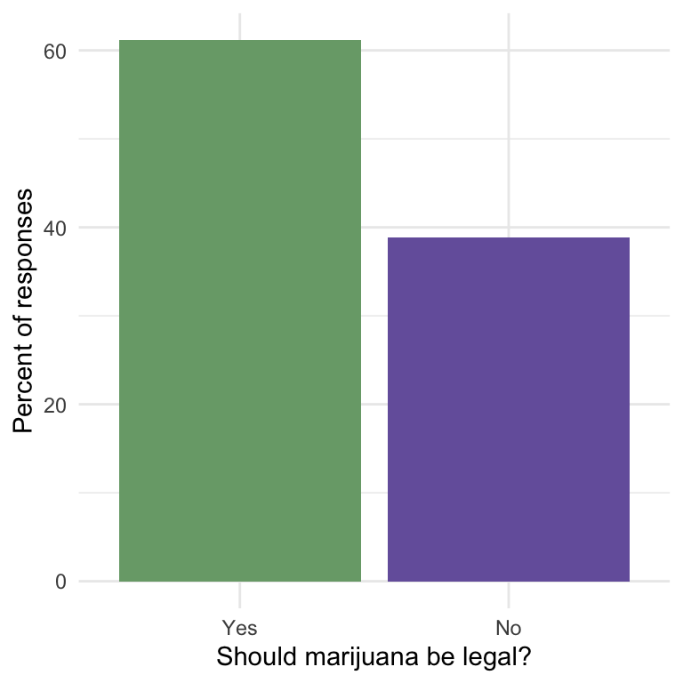
I changed the code slightly because of two warnings. Newer versions of {ggplot2} have deprecated some older functions:
..count..) was deprecated in {ggplot2} version 3.4.0. Please use after_stat(count) instead.guide argument in scale_*() cannot be FALSE. This was deprecated in {ggplot2} version 3.3.4. Please use “none” instead. (I have slightly edited both warnings)Compare the reproduction with the original Graph 1.1 (a).
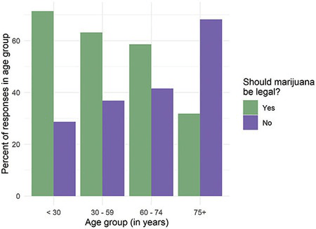
R Code 1.5 b: Reproducing bar chart Figure 1.2 using geom_col()
gss_2016_clean <-  base::readRDS("data/chap01/gss_2016_clean.rds")

## create figure 1.2 ########
gss_2016_clean |>
  dplyr::group_by(grass, age_cat) |>
  dplyr::count() |>
  dplyr::group_by(age_cat) |>
  dplyr::mutate(perc_grass = 100 * n / base::sum(n)) |>
  ggplot2::ggplot(ggplot2::aes(x = age_cat, fill = grass,
             y = perc_grass)) +
  ggplot2::geom_col(position = 'dodge') +
  ggplot2::theme_minimal() +
  ggplot2::scale_fill_manual(values = c('#79a778', '#7662aa'),
                    name = "Should marijuana\nbe legal?") +
  ggplot2::labs(x = "Age group (in years)",
       y = "Percent of responses in age group")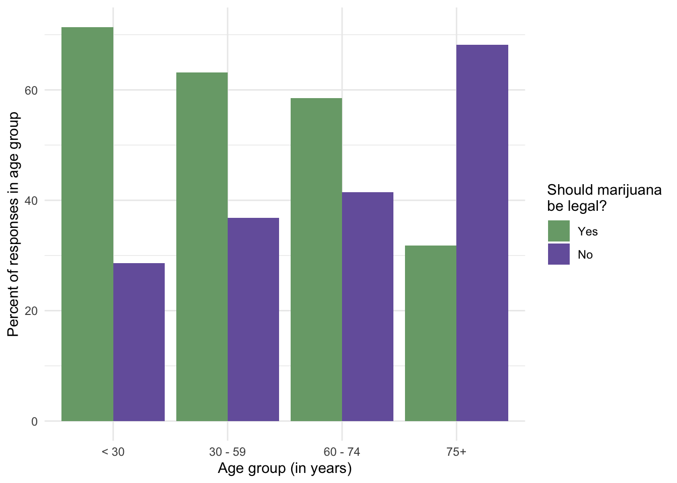
Graph 1.2 uses ggplot2::geom_bar() whereas this figure here calls the ggplot2::geom_col() function.
There are two types of bar charts:
geom_bar()andgeom_col().geom_bar()makes the height of the bar proportional to the number of cases in each group … . If you want the heights of the bars to represent values in the data, usegeom_col()instead.geom_bar()usesstat_count()by default: it counts the number of cases at each x position.geom_col()usesstat_identity(): it leaves the data as is. (Bar charts with {ggplot2})
Compare the reproduction with the original Graph 1.1 (b).
Exercises for the Coder & Hacker edition
SwR objectives
nhanes_2013_ch1.csv with the book materials at edge.sagepub.com/harris1e (Achievement 1) (Section 1.6.3 in tab “read_csv()”)age_cat with 4 categories: 18–29, 30–39, 40–49, 50–59 (Achievement 7) (Section 1.6.5 in tab “Numbers”)My own additional exercises
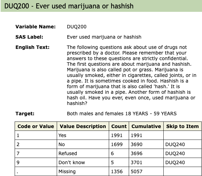
Use the National Health and Nutrition Examination Survey (NHANES) data to examine marijuana use in the United States. Spend a few minutes looking through the NHANES website (https://www.cdc.gov/nchs/nhanes/index.htm) before you begin, including finding the online codebook for the 2013–2014 data. Complete the following tasks to explore whether age is related to marijuana use in the United States.
The 2013–2014 codebook is on the page NHANES 2013-2014. On this page are the links to different types of data, documentations or codebooks.
You can choose from
Bullet List: NHANES has six different data sections
Clicking of one of these links opens a page where a table contains the following information:
Bullet List: NHANES data pages has download links for documentation and data files
Datasets and Documentation and Frequently Asked Questions (FAQs) are important introductory pages.
NHANES data are saved in a SAS transport (.XPT) file. These file can be read with foreign::read.xport() and haven::read_xpt(). There is also a page with example code to download/import NHANES data files. I will use {haven} instead of the recommended {foreign} package.
Experiment 1.1 : Download and work with NHANES SAS .xpt file data (Demo)
R Code 1.6 : Save a SAS transport (.xpt) file from the NHANES site for demo purposes and display the structure of the file
## download only once (manually)
utils::download.file(
    "https://wwwn.cdc.gov/Nchs/Nhanes/2017-2018/P_BPXO.XPT",
    tf <- base::tempfile(),
    mode = "wb"
)
blood_pressure_demo <- haven::read_xpt(tf)

save_data_file("chap01", blood_pressure_demo, "blood_pressure_demo.rds")(This code chunk has no visible output)
With the exception of using (haven) instead of {foreign}, I followed the instruction from the NHANES recommendation. We see labelled data as it was expected from the import with {haven}.
In Listing / Output 1.10 I have already used the utils::download.file() function: There are some differences:
.zip file, therefore I used unz() to unzip the file and to read haven::read_dta() instead haven::read_xpt().base::unlink(temp) command to unlink the temporary file, which is not done here.mode = "wb" for writing binary files. As I understood this is only important for Windows user. On my Mac I could stick with the default value mode = "w". But for reproducibility it would be better to use in the future the more general option with mode = "wb".Package {nhanesA} facilitates downloading NHANES data
I just learned that there is a {nhanesA} package that facilitates downloading data to R. (2024-01-20) The latest package release is brand-new (2024-01-09).
I am planning to use this package when I am working with again with NHANES data in Chapter 6. Just for me to remember:
R Code 1.7 : Show data summary of three blood pressure variables with utils::str() (Demo)
#> tibble [11,656 × 3] (S3: tbl_df/tbl/data.frame)
#>  $ BPAOARM: chr [1:11656] "R" "R" "R" "R" ...
#>   ..- attr(*, "label")= chr "Arm selected - oscillometric"
#>  $ BPXOSY1: num [1:11656] 109 99 123 102 116 138 104 100 141 NA ...
#>   ..- attr(*, "label")= chr "Systolic - 1st oscillometric reading"
#>  $ BPXODI1: num [1:11656] 67 56 73 65 68 70 58 64 77 NA ...
#>   ..- attr(*, "label")= chr "Diastolic - 1st oscillometric reading"
R Code 1.8 : Show data summary of three blood pressure variables with summary() (Demo)
#>    BPAOARM             BPXOSY1        BPXODI1
#>  Length:11656       Min.   : 52    Min.   : 31.00
#>  Class :character   1st Qu.:106    1st Qu.: 63.00
#>  Mode  :character   Median :117    Median : 71.00
#>                     Mean   :120    Mean   : 72.04
#>                     3rd Qu.:130    3rd Qu.: 80.00
#>                     Max.   :225    Max.   :151.00
#>                     NA's   :1304   NA's   :1304
R Code 1.9 : Show data summary of three blood pressure variables with skim() (Demo)
| Name | dplyr::select(blood_press… |
| Number of rows | 11656 |
| Number of columns | 3 |
| _______________________ | |
| Column type frequency: | |
| character | 1 |
| numeric | 2 |
| ________________________ | |
| Group variables | None |
Variable type: character
| skim_variable | n_missing | complete_rate | min | max | empty | n_unique | whitespace |
|---|---|---|---|---|---|---|---|
| BPAOARM | 0 | 1 | 0 | 1 | 2152 | 3 | 0 |
Variable type: numeric
| skim_variable | n_missing | complete_rate | mean | sd | p0 | p25 | p50 | p75 | p100 | hist |
|---|---|---|---|---|---|---|---|---|---|---|
| BPXOSY1 | 1304 | 0.89 | 120.00 | 19.95 | 52 | 106 | 117 | 130 | 225 | ▁▇▅▁▁ |
| BPXODI1 | 1304 | 0.89 | 72.04 | 12.42 | 31 | 63 | 71 | 80 | 151 | ▁▇▃▁▁ |
R Code 1.10 : Show some blood pressure data with my private function my_glance_data()
#> # A tibble: 10 × 4
#>      obs arm_selected systolic diastolic
#>    <int> <chr>           <dbl>     <dbl>
#>  1     1 R                 109        67
#>  2   356 R                 131        64
#>  3  1252 R                 100        54
#>  4  2369 R                 173        82
#>  5  5273 R                 131        77
#>  6  8826 R                 111        74
#>  7  9290 R                 112        69
#>  8 10289 R                 141        74
#>  9 10801 R                 112        71
#> 10 11656 R 122 55Exercise 1.1 : Coder exercises: Import & clean data
R Code 1.11 : Open the 2013–2014 NHANES data file that comes with the book
## load and save it only once (manually) ########
nhanes_2013 <- readr::read_csv("data/chap01/nhanes_2013_ch1.csv")
save_data_file("chap01", nhanes_2013, "nhanes_2013.rds")(This R Code chunk has no visible output.)
R Code 1.12 : Look at the data with utils::str() and skimr::skim()
#>       ...1          DUQ200        RIDAGEYR        RIAGENDR
#>  Min.   :   1   Min.   :1.00   Min.   :18.00   Min.   :1.000
#>  1st Qu.:1265   1st Qu.:1.00   1st Qu.:30.00   1st Qu.:1.000
#>  Median :2529   Median :1.00   Median :42.00   Median :2.000
#>  Mean   :2529   Mean   :1.48   Mean   :42.49   Mean   :1.522
#>  3rd Qu.:3793   3rd Qu.:2.00   3rd Qu.:56.00   3rd Qu.:2.000
#>  Max.   :5057   Max.   :9.00   Max.   :69.00   Max.   :2.000
#> NA's :1356utils::str(nhanes_2013)#> spc_tbl_ [5,057 × 4] (S3: spec_tbl_df/tbl_df/tbl/data.frame)
#> $ ...1 : num [1:5057] 1 2 3 4 5 6 7 8 9 10 ...
#> $ DUQ200 : num [1:5057] NA 1 1 NA 1 NA 2 2 1 2 ...
#> $ RIDAGEYR: num [1:5057] 69 54 56 61 56 65 26 33 32 18 ...
#> $ RIAGENDR: num [1:5057] 1 1 1 2 2 1 2 2 1 1 ...
#> - attr(*, "spec")=
#> .. cols(
#> .. ...1 = col_double(),
#> .. DUQ200 = col_double(),
#> .. RIDAGEYR = col_double(),
#> .. RIAGENDR = col_double()
#> .. )
#> - attr(*, "problems")=<externalptr>skimr::skim(nhanes_2013)| Name | nhanes_2013 |
| Number of rows | 5057 |
| Number of columns | 4 |
| _______________________ | |
| Column type frequency: | |
| numeric | 4 |
| ________________________ | |
| Group variables | None |
Variable type: numeric
| skim_variable | n_missing | complete_rate | mean | sd | p0 | p25 | p50 | p75 | p100 | hist |
|---|---|---|---|---|---|---|---|---|---|---|
| …1 | 0 | 1.00 | 2529.00 | 1459.97 | 1 | 1265 | 2529 | 3793 | 5057 | ▇▇▇▇▇ |
| DUQ200 | 1356 | 0.73 | 1.48 | 0.61 | 1 | 1 | 1 | 2 | 9 | ▇▁▁▁▁ |
| RIDAGEYR | 0 | 1.00 | 42.49 | 15.16 | 18 | 30 | 42 | 56 | 69 | ▇▆▇▆▇ |
| RIAGENDR | 0 | 1.00 | 1.52 | 0.50 | 1 | 1 | 2 | 2 | 2 | ▇▁▁▁▇ |
utils::str() and skimr::skim()
As one of the packages for displaying summaries I am using the {skimr} package (see Section A.84).
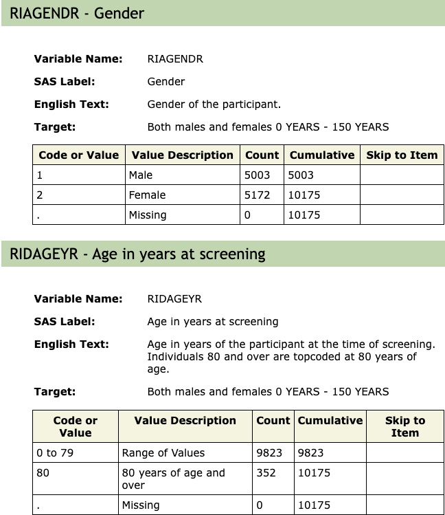
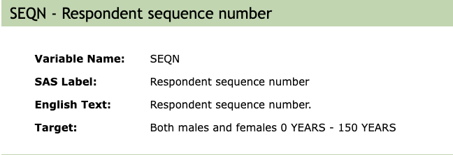
Unfortunately the .csv files does not include labelled data. Therefore I had to look for the variable names in all different NHANES sections as outlined in Bullet List 1.1. Inspecting the accompanying NHANES download pages (see: Bullet List 1.2) I could look for the variable names in the download links for the documentation.
There is an additional column ...1 (see Listing / Output 1.6) providing row numbers. Maybe this column works as an ID, a kind sequence number, so that one could merge other data files identified by this number. (See SEQN: Respondent Sequence Number). Why this column has lost its name, I do not know. Perhaps it has to do with the data import done by the book author?
To facilitate the work I made screenshots from these four variables:
R Code 1.13 : Look at the data after data cleaning
nhanes_2013 <- base::readRDS("data/chap01/nhanes_2013.rds")

nhanes_2013_clean <- nhanes_2013 |>
    dplyr::rename(nr = ...1) |>
    dplyr::rename(
        sex = RIAGENDR,
        age = RIDAGEYR,
        grass = DUQ200
        ) |>
    dplyr::mutate(grass =
          dplyr::na_if(x = grass, y = 7)) |>
    dplyr::mutate(grass =
          dplyr::na_if(x = grass, y = 9)) |>
    tidyr::drop_na() |>
    dplyr::mutate(sex = forcats::as_factor(sex)) |>
    dplyr::mutate(grass = forcats::as_factor(grass)) |>
    dplyr::mutate(grass =
          forcats::fct_recode(grass,
          "Yes" = "1", "No" = "2")) |>
    dplyr::mutate(sex =
          forcats::fct_recode(sex,
          "Male" = "1", "Female" = "2"))

## save cleaned data ###############
save_data_file("chap01", nhanes_2013_clean, "nhanes_2013_clean.rds")

base::summary(nhanes_2013_clean)
#> nr grass age sex
#> Min. : 2 Yes:1991 Min. :18.00 Male :1792
#> 1st Qu.:1288 No :1699 1st Qu.:26.00 Female:1898
#> Median :2546 Median :38.00
#> Mean :2536 Mean :37.48
#> 3rd Qu.:3784 3rd Qu.:48.00
#> Max. :5056 Max. :59.00skimr::skim(nhanes_2013_clean)| Name | nhanes_2013_clean |
| Number of rows | 3690 |
| Number of columns | 4 |
| _______________________ | |
| Column type frequency: | |
| factor | 2 |
| numeric | 2 |
| ________________________ | |
| Group variables | None |
Variable type: factor
| skim_variable | n_missing | complete_rate | ordered | n_unique | top_counts |
|---|---|---|---|---|---|
| grass | 0 | 1 | FALSE | 2 | Yes: 1991, No: 1699 |
| sex | 0 | 1 | FALSE | 2 | Fem: 1898, Mal: 1792 |
Variable type: numeric
| skim_variable | n_missing | complete_rate | mean | sd | p0 | p25 | p50 | p75 | p100 | hist |
|---|---|---|---|---|---|---|---|---|---|---|
| nr | 0 | 1 | 2535.51 | 1450.33 | 2 | 1288.25 | 2546.5 | 3784.25 | 5056 | ▇▇▇▇▇ |
| age | 0 | 1 | 37.48 | 12.43 | 18 | 26.00 | 38.0 | 48.00 | 59 | ▇▆▆▆▆ |
Recoded gender to sex
In all R code chunks and text passages I have changed the gender category to sex. “Sex” refers only to biology but “gender” is a broader concepts: It refers to identity construction, that include biological, psycho-social, and cultural factors.
Gender refers to the characteristics of women, men, girls and boys that are socially constructed. This includes norms, behaviours and roles associated with being a woman, man, girl or boy, as well as relationships with each other. As a social construct, gender varies from society to society and can change over time. … Gender interacts with but is different from sex, which refers to the different biological and physiological characteristics of females, males and intersex persons, such as chromosomes, hormones and reproductive organs. Gender and sex are related to but different from gender identity. Gender identity refers to a person’s deeply felt, internal and individual experience of gender, which may or may not correspond to the person’s physiology or designated sex at birth. (WHO)
My learning from the above procedure of data cleaning
...1 into accents.dplyr::rename() but not for dplyr::na_if() and forcats::as_factor() because here we need to change the column values with the command.dplyr::na_if()
tidyr::drop_na().forcats::as_factor() needs to rewrite the column as factor with dplyr::mutate()
Exercise 1.2 : Bar chart (with different bar width ans space) showing the percentage of NHANES participants answering yes and no to marijuana use
R Code 1.14 : Show frequencies and percentages of NHANES participants answering yes and no to “Ever used marijuana or hashish”
#> # A tibble: 2 × 3
#>   `Ever used grass or hash` Freq        Perc
#>   <chr>                     <table[1d]> <table[1d]>
#> 1 Yes                       1991        53.96
#> 2 No                        1699        46.04
Instead of using name and value I could have used the position of the column numbers 1 and 2 (all names without the `-sign.)
This is a manual calculation using the {tidyverse} approach: I am sure there are some packages that may facilitate this computation (e.g., {Janitor} or {DescTools}), but I had difficulties to apply the appropriate functions.
R Code 1.15 : Percentage of NHANES participants answering yes and no to marijuana use
nhanes_2013_clean <- base::readRDS("data/chap01/nhanes_2013_clean.rds")

ggplot2::ggplot(nhanes_2013_clean,
    ggplot2::aes(grass,
         y = 100 * ggplot2::after_stat(count) /
             base::sum(ggplot2::after_stat(count)),
             fill = grass
        )) +
    ggplot2::geom_bar() +
    ggplot2::theme_minimal() +
    ggplot2::scale_fill_manual(values = c("darkgreen", 'darkred'),
                    guide = "none") +
    ggplot2::scale_y_continuous(
        breaks = base::seq(0, 50, by = 10),
        labels = scales::label_percent(scale = 1)) +
    ggplot2::labs(x = "Did you ever use marijuana or hashish?",
y = "Percent of responses") 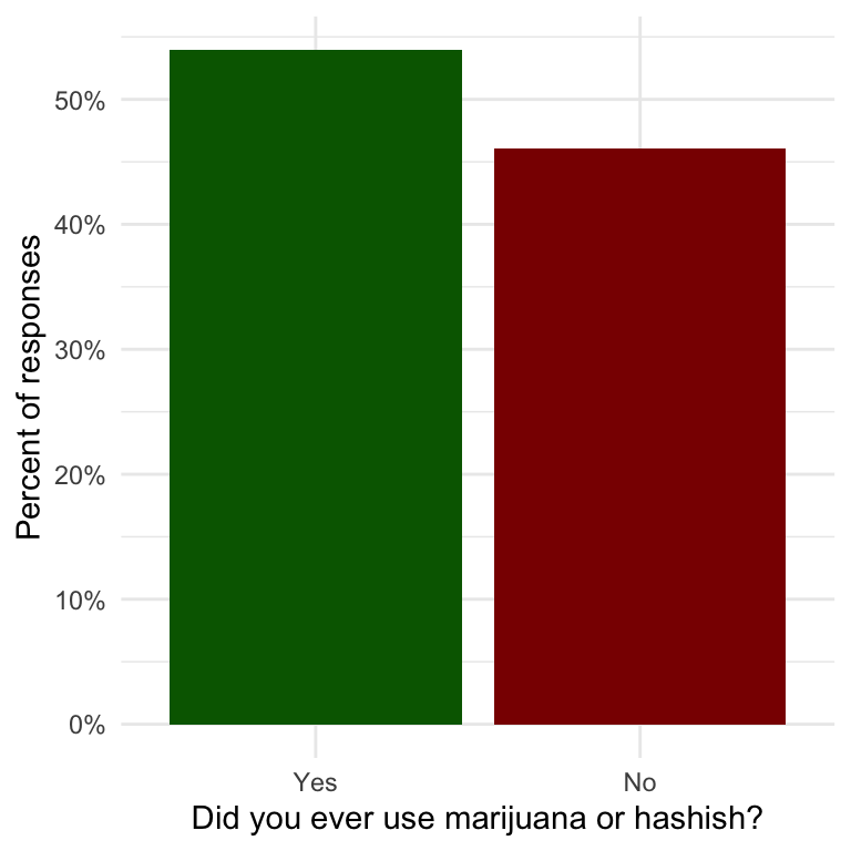
The bars are very thick. I tried with ggplot2::geom_bar(width = 0.5) to make them thinner. But I failed. (See Listing / Output 1.7)
R Code 1.16 : Percentage of NHANES participants answering yes and no to marijuana use
nhanes_2013_clean <- base::readRDS("data/chap01/nhanes_2013_clean.rds")

ggplot2::ggplot(nhanes_2013_clean,
    ggplot2::aes(grass,
         y = 100 * ggplot2::after_stat(count) /
             base::sum(ggplot2::after_stat(count)),
             fill = grass
        )) +

    ## provide thinner bars, standard = 0.9
    ggplot2::geom_bar(width = 0.5) +

    ggplot2::theme_minimal() +
    ggplot2::scale_fill_manual(values = c("darkgreen", 'darkred'),
                    guide = "none") +
    ggplot2::scale_y_continuous(
        breaks = base::seq(0, 50, by = 10),
        labels = scales::label_percent(scale = 1)) +
    ggplot2::labs(x = "Did you ever use marijuana or hashish?",
y = "Percent of responses") 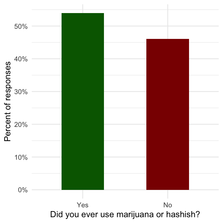
The bars are now thin but the space between didn’t change. I tried several options with the position argument to adjust bar width and spacing:
Dodging preserves the vertical position of an geom while adjusting the horizontal position. position_dodge() requires the grouping variable to be be specified in the global or geom_* layer. Unlike position_dodge(), position_dodge2() works without a grouping variable in a layer. position_dodge2() works with bars and rectangles, but is particulary useful for arranging box plots, which can have variable widths.
All my trials with position_dodge() and position_dodge2() failed. The only two strategies I could reduce the spacing was:
R Code 1.17 : Percentage of NHANES participants answering yes and no to marijuana use
nhanes_2013_clean <- base::readRDS("data/chap01/nhanes_2013_clean.rds")

ggplot2::ggplot(nhanes_2013_clean,
    ggplot2::aes(grass,
         y = 100 * ggplot2::after_stat(count) /
             base::sum(ggplot2::after_stat(count)),
             fill = grass
        )) +
    ggplot2::geom_bar() +
    ggplot2::theme_minimal() +
    ggplot2::scale_fill_manual(values = c("darkgreen", 'darkred'),
                    guide = "none") +
    ggplot2::scale_y_continuous(
        # n.breaks = 10,
        breaks = base::seq(0, 50, by = 5),
        labels = scales::label_percent(scale = 1)) +
    ggplot2::labs(x = "Did you ever use marijuana or hashish?",
       y = "Percent of responses") +
    ggplot2::theme(aspect.ratio = 3/1)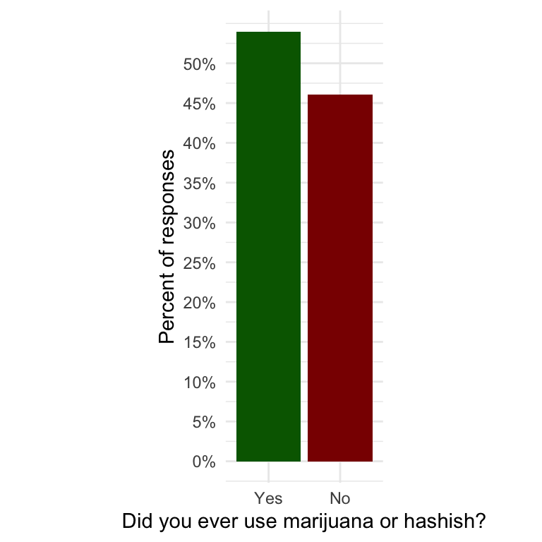
What I learned from creating the bar chart
Even with this simple example of a bar chart I learned some new options:
ggplot2::after_stat() inside the aesthetics of the first layer to convert frequencies to percentages.n.breaks = <number> or breaks = base::seq(from, to, by = <number>) inside the appropriate scale.%-sign after the values. As I have already calculated the percentages I need to reduce the default value of scale = 100 to scale = 1.ggplot2::theme(aspect.ratio = <number>/1) creating thinner bars and reducing the spacing between the bars accordingly. In my case I changed the aspect ratio to 3/1. A bigger front number compresses the graph, a smaller front number extends it. Aspect ratio of 1/1 is the standard (= no change).Exercise 1.3 : Exploring the percentage of NHANES participants answering yes or no to marijuana use by age category and sex
R Code 1.18 : Show frequencies and percentages of NHANES participants answering yes and no to “Ever used marijuana or hashish”
nhanes_2013_clean <- base::readRDS("data/chap01/nhanes_2013_clean.rds")

nhanes_2013_grouped <- nhanes_2013_clean |>
    ## cut age into several defined age groups
    dplyr::mutate(age_cat = base::cut(age,
                   breaks = c(-Inf, 29, 39, 49, 59),
                   labels = c("18 - 29", "30 - 39", "40 - 49", "50 - 59"))) |>
    dplyr::select(grass, sex, age_cat)


## older trial, without the knowledge of {gtsummary}
# tibble::enframe(table(nhanes_2013_grouped$age_cat)) |>
#     dplyr::rename(`Ever used grass or hash` = 1, Freq = 2) |>
#     dplyr::mutate(Perc = round(100 * Freq / sum(Freq), 2))

nhanes_2013_grouped |>
    labelled::set_variable_labels(
        grass = "Ever used grass or hash?"
    ) |>
    gtsummary::tbl_summary(
        label = list(
            age_cat = "Age Category",
            sex = "Sex"
        ),
        type = grass ~ "categorical"
    ) |>
    gtsummary::bold_labels()

save_data_file("chap01", nhanes_2013_grouped, "nhanes_2013_grouped.rds")| Characteristic | N = 3,6901 |
|---|---|
| Ever used grass or hash? | |
| Yes | 1,991 (54%) |
| No | 1,699 (46%) |
| Sex | |
| Male | 1,792 (49%) |
| Female | 1,898 (51%) |
| Age Category | |
| 18 - 29 | 1,154 (31%) |
| 30 - 39 | 859 (23%) |
| 40 - 49 | 855 (23%) |
| 50 - 59 | 822 (22%) |
| 1 n (%) | |
Instead of using 1 and 2 I could have used the position of the column numbers name and value (all names without the `-sign.)
This is a manual calculation using the {tidyverse} approach: I am sure there are some packages that may facilitate this computation (e.g., {Janitor} or {DescTools}), but I had difficulties to apply the appropriate functions.
R Code 1.19 : Table: Percentage of NHANES participants by age group answering yes and no to marijuana use in percent of total responses
nhanes_2013_grouped <- base::readRDS("data/chap01/nhanes_2013_grouped.rds")

nhanes_2013_grouped |>
    labelled::set_variable_labels(
        grass = "**Ever used grass or hash?**"
    ) |>
    gtsummary::tbl_cross(
        label = list(
            age_cat = "Age Category",
            sex = "Sex"
        ),
        row = age_cat,
        col = grass,
        percent = "cell"
    ) |>
    gtsummary::modify_header(
      stat_1 = '**Yes**',
      stat_2 = '**No**',
      stat_0 = '**Total**'
    ) |>
    gtsummary::bold_labels()
Ever used grass or hash?
|
Total | ||
|---|---|---|---|
| Yes | No | ||
| Age Category | |||
| 18 - 29 | 662 (18%) | 492 (13%) | 1,154 (31%) |
| 30 - 39 | 466 (13%) | 393 (11%) | 859 (23%) |
| 40 - 49 | 405 (11%) | 450 (12%) | 855 (23%) |
| 50 - 59 | 458 (12%) | 364 (9.9%) | 822 (22%) |
| Total | 1,991 (54%) | 1,699 (46%) | 3,690 (100%) |
I have required {gtsummary} to calculate the percentage with one decimal place. The reason was that the graphic did not match the table. For instance: Without decimal places the “No”-proportion of the age group 18-29 was with 13% equal to the “Yes”-proportion of the age group 30-39. But in the figure these two bars have a different height. The reason was a rounding error: Both values 13.3% and 12.6% were rounded to 13%. But in the figure one could see the difference of 0.7% in the length of the bars.
R Code 1.20 : Figure: Percentage of NHANES participants by age group answering yes and no to marijuana use in percent of total responses
## age groups bar chart 1 ########
nhanes_2013_grouped |>
    ggplot2::ggplot(ggplot2::aes(
        x = age_cat,
        fill = grass,
         y = 100 * ggplot2::after_stat(count) /
             base::sum(ggplot2::after_stat(count))
        )
    ) +
    ggplot2::geom_bar(position = 'dodge') +
    ggplot2::theme_minimal() +
    ggplot2::scale_fill_manual(values = c('darkgreen', 'darkred'),
                    name = "Ever used\ngrass or hash?") +
    ggplot2::labs(x = "Age group (in years)",
       y = "Percent of total responses")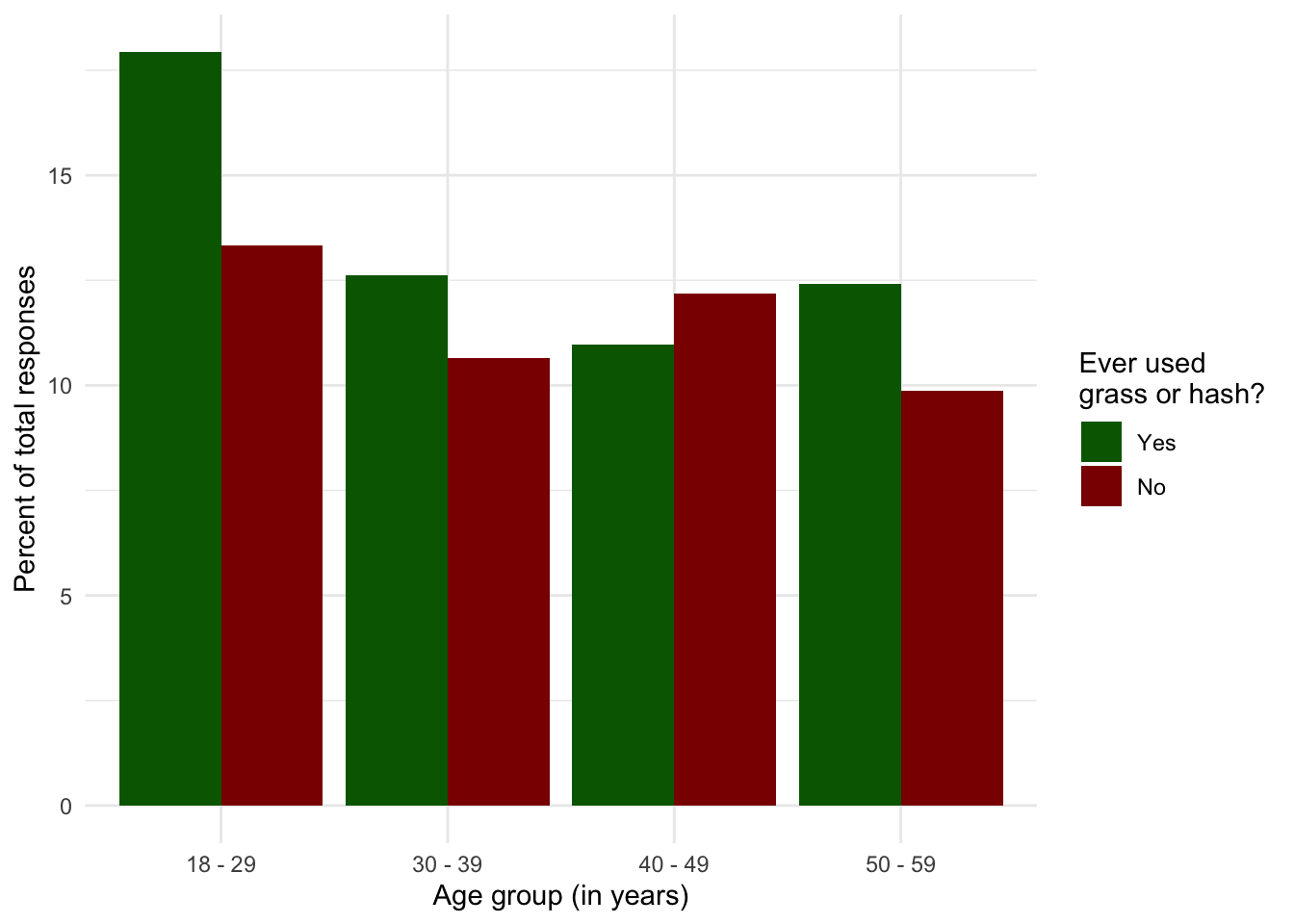
R Code 1.21 : Table:: Percentage of NHANES 2013 survey participants by age group answering yes and no to marijuana use in percent of age group
nhanes_2013_grouped <- base::readRDS("data/chap01/nhanes_2013_grouped.rds")

nhanes_2013_grouped |>
    labelled::set_variable_labels(
            grass = "**Ever used grass or hash?**"
        ) |>
    gtsummary::tbl_cross(
        label = list(
            age_cat = "Age Category",
            sex = "Sex"
        ),
        row = age_cat,
        col = grass,
        percent = "row",
        margin = "column",
        digits = c(0, 1)
    ) |>
    gtsummary::modify_header(
      stat_1 = '**Yes**',
      stat_2 = '**No**',
      stat_0 = '**Total**'
    ) |>
    gtsummary::bold_labels()
Ever used grass or hash?
|
Total | ||
|---|---|---|---|
| Yes | No | ||
| Age Category | |||
| 18 - 29 | 662 (57.4%) | 492 (42.6%) | 1,154 (100.0%) |
| 30 - 39 | 466 (54.2%) | 393 (45.8%) | 859 (100.0%) |
| 40 - 49 | 405 (47.4%) | 450 (52.6%) | 855 (100.0%) |
| 50 - 59 | 458 (55.7%) | 364 (44.3%) | 822 (100.0%) |
R Code 1.22 : Figure: Percentage of NHANES participants of the 2013 survey answering yes and no to marijuana use in percent of age group
## age groups bar chart 2 ########
nhanes_2013_grouped |>
  dplyr::group_by(grass, age_cat) |>
  dplyr::count() |>
  dplyr::group_by(age_cat) |>
  dplyr::mutate(perc_grass = 100 * n / base::sum(n)) |>
  ggplot2::ggplot(ggplot2::aes(x = age_cat, fill = grass,
             y = perc_grass)) +
  ggplot2::geom_col(position = 'dodge') +
  ggplot2::theme_minimal() +
  ggplot2::scale_fill_manual(values = c('darkgreen', 'darkred'),
                    name = "Ever used\ngrass or hash?") +
  ggplot2::labs(x = "Age group (in years)",
       y = "Percent of responses in age group")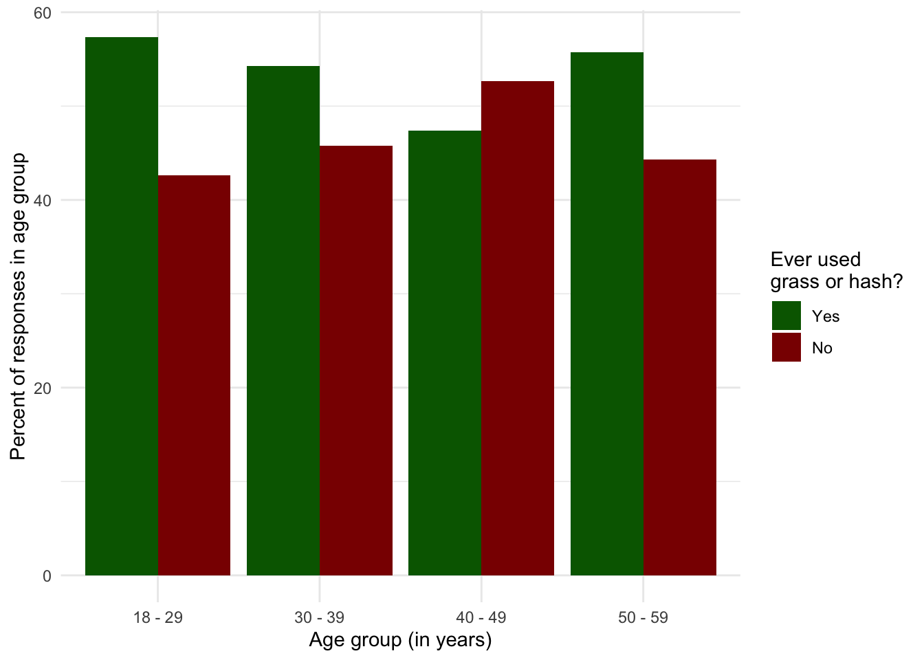
R Code 1.23 : Percentage of NHANES participants 2013 survey by age group and sex answering yes and no to marijuana use
nhanes_2013_grouped <-
    base::readRDS("data/chap01/nhanes_2013_grouped.rds")

## age and sex bar chart ########
nhanes_2013_grouped |>
  dplyr::group_by(grass, age_cat, sex) |>
  dplyr::count() |>
  dplyr::group_by(age_cat, sex) |>
  dplyr::mutate(perc_grass_2 = 100 * n / base::sum(n)) |>
  ggplot2::ggplot(ggplot2::aes(
      x = age_cat,
      y = perc_grass_2,
      fill = sex)) +
  ggplot2::geom_col(position = 'dodge') +
  ggplot2::theme_minimal() +
  ggplot2::scale_fill_manual(values = c('#f98e31', '#730b6d'),
                             name = "sex") +
  ggplot2::labs(
          x = "Age group (in years)",
          y = "Percent of males/females that used marijuana or hashish"
      )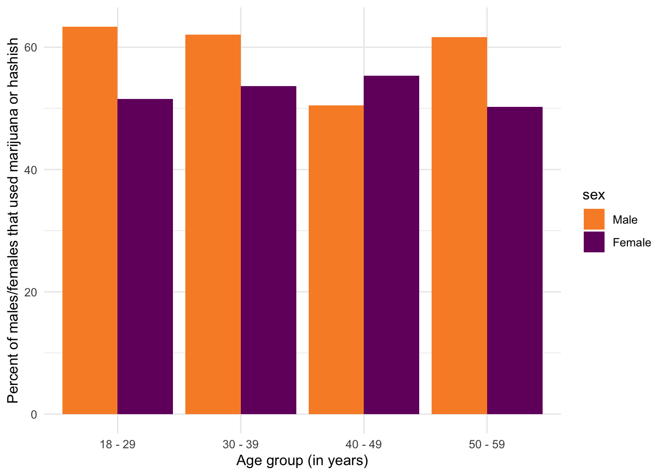
With the exception of the oldest age group the graphic shows that the proportion of marijuana / hashish user increases with younger people. One possible explanation for the untypical high use in the oldest age group could be that people between 50-59 of the 2013 survey were born between 1954-1963 and were young adults during the time of the Flower Power generation part of the counterculture of the 1960s-1970s.
Graph 1.7 is a little difficult to interpret. Both bars colors shows the proportion of “Yes”-respondents in the appropriate age group. For instance: About 62% of males and about 51% of women of the age group 18-29 said “Yes”.
Therefore the bars to not sum up to 100%. The figures shows only the “Yes” part of the dichotomous grass variable for men and women in a certain age group. The other “No” part is missing.
To distinguish the sex colors in Graph 1.7 from the Yes/No colors in Graph 1.5 and Graph 1.6 I chose at first some kind of blue for men and red for females. But I learned from An alternative to pink & blue: Colors for gender data that one should avoid this stereotypical colors.
In our western culture, these colors come with the whole gender stereotype baggage. Pink means weak, shy girls who play with dolls and don’t deserve as much as boys. Blue stands for boys who need to be strong & rough. When we create a chart with pink & blue, we endorse gender stereotypes.
Graph 1.3 with GSS data 2016 shows that younger people support the legalizing of marijuana. Therefore we can expect that in the future the proportion of people that approve legalizing will increase. With a small project on my own I have backed up this thesis. Graph 1.12 demonstrates that the percentage of supporters has increased very strongly in the last years and has now hit the 70% mark. This trend is very clear even I have not distinguished in the longitudinal study between different age groups.
The graphs of the NHANES 2013 data in Graph 1.5 and fig-grass-age-group2 show that the highest proportion of people ever used marijuana or hashish lies in youngest age. The age trend is not very clear, because we have only figures for person equal or under 59 years. (Here would be necessary another small project with longitudinal analysis including newer data.)
With the exception of the age group 40-49 the proportion of males ever used in their respective age group is higher than the percentage of women. (See Graph 1.7). But this is only a snapshot and difficult to interpret. Another possible thesis could be that there is a tiny upward trend from old top young in marijuana use. One possible explanation for the untypical higher use in the oldest age group could be that people between 50-59 of the 2013 survey were born between 1954-1963 and were young adults during the time of the Flower Power generation part of the counterculture of the 1960s-1970s.
I am very interested how to get GSS data directly from the GSS website, so that I could work on interesting research questions myself.
I have found several resources helping to work with the GSS. The most important one is the {gssr} package (see: Section A.35)
Resource 1.2 : asdfree: Analyze Survey Data for Free
Analyze Survey Data for Free is a bookdown website by Anthony Damico with currently 64 locations to grab free survey data. As expected it features also a description of the GSS including analysis examples with the {survey} package and — especially important for my purpose here — {lodown}, a package on GitHub that is not maintained anymore.
Experiment 1.2 features five different strategies to download GSS data:
Experiment 1.2 : How to get the General Social Survey (GSS) data
To use all the facilities of the GSS Data Explorer (tagging, tabulating, data extracting) you need to register for a free account. The good thing is: This is a onetime procedure.
Procedure 1.1 : Downloading data extracts with the GSS Data Explorer
As one can see this is a somewhat cumbersome procedure to download the desired data. Following the proposed strategies in the other tabs are much easier for importing GSS data. But using the GSS Data Explorer is very helpful to explore the dataset. Apply the first three steps of the above list to find the correct variable names, to read the exact wording of the question asked and to inspect the different codes that are used for the variable. Otherwise you have to skim the more than 700 pages of the GSS codebook.😭
Another approach is to download the complete dataset (or all variables of those years you are interested in) and manage the data in such a way that it can be easily used for your research question. (See Section 1.4)
Procedure 1.2 : Download GSS individual year data sets (cross-section only)
2016 in our case) under the section “Individual Year Data Sets (cross-section only)” and download the file 2016_stata.zip (994 MB) into your preferred folder on your hard disk. After you extract the .zip file you will get the STAT file GSS2016.dta (4.4 MB).R Code 1.24 : Import STATA GSS 2016 file into R using (haven)
## run only once (manually) ###########
gss_2016_man <- haven::read_dta("data/chap01/GSS2016.dta")
save_data_file("chap01", gss_2016_man, "gss_2016_man.rds")(This R code chunk has no visible output)
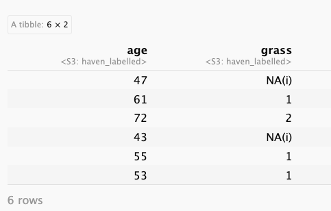
#> # A tibble: 10 × 3
#>      obs age       grass
#>    <int> <dbl+lbl> <dbl+lbl>
#>  1     1 47        NA(i) [iap]
#>  2   172 27            1 [should be legal]
#>  3   562 70            2 [should not be legal]
#>  4   898 60            2 [should not be legal]
#>  5  1019 30            1 [should be legal]
#>  6  1176 80            2 [should not be legal]
#>  7  1505 53        NA(i) [iap]
#>  8  1911 54            2 [should not be legal]
#>  9  2622 62        NA(i) [iap]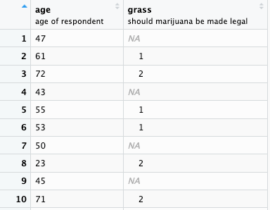
#> 10 2867 72 2 [should not be legal]{haven} imports data as labelled vectors
The data structure we have found here is very different from the Excel data file provided with the book.
Labelled vectors is a completely new feature for me. I learned that value labels and other metadata tags that are commonly seen when working with other statistical software like SAS, STATA or SPSS (cf. Survey Research and Datasets in R, here section 3 Labelled Data)
A labelled vector is a common data structure in other statistical environments, allowing you to assign text labels to specific values. This class makes it possible to import such labelled vectors in to R without loss of fidelity. (Create a labelled vector)
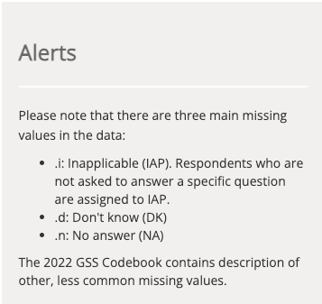
I will go into more details in Section 1.8. The important thing here is to notice that the variable grass has labelled values that explain the short code. Code 1 represents the respondent option that marijuana should be legalized and 2 the opposite. We also learn that there is with NA i a special kind of NA value:
.i: Inapplicable (IAP). Respondents who are not asked to answer a specific question are assigned to IAP. (See Alert on the STATA download page)
On the website we see under the “Alert” section that there other kind of NA’s as well. And the 2022 GSS Codebook describes still other, less common missing values.
Additional comments
I chose for file saving the base::saveRDS() option (and not base::save()) because when later reading into R again with base::readRDS() it does not overwrite a variable with the same name respectively I can assign the file to another variable name.
R Code 1.25 : Get year 2016 of GSS data set with base::download.file()
## run only once (manually) ###########
temp <- base::tempfile()
utils::download.file("https://gss.norc.org/documents/stata/2016_stata.zip",temp)
gss_2016_aut <- haven::read_dta(base::unz(temp, "GSS2016.dta"))
base::unlink(temp)
save_data_file("chap01", gss_2016_aut, "gss_2016_aut.rds")base::download.file()
(This R code chunk has no visible output)
This time we have the file downloaded programmatically which is much better in term of reproducibility. We don’t need now to import the data {haven} but can call base::readRDS().
#> # A tibble: 10 × 3
#>      obs age       grass
#>    <int> <dbl+lbl> <dbl+lbl>
#>  1     1 47        NA(i) [iap]
#>  2   172 27            1 [should be legal]
#>  3   562 70            2 [should not be legal]
#>  4   898 60            2 [should not be legal]
#>  5  1019 30            1 [should be legal]
#>  6  1176 80            2 [should not be legal]
#>  7  1505 53        NA(i) [iap]
#>  8  1911 54            2 [should not be legal]
#>  9  2622 62        NA(i) [iap]
#> 10 2867 72 2 [should not be legal].rds file into R and glance at the data
Data now have a more R like appearance, even if the variable classes with 1 and 2 mean.
The following strategy I have taken from the bookdown book Analyze Survey Data for Free (asdf.com) It gives step by step instructions to explore public Microdata. Here I refer to the General Social Survey (GSS) section of the book.
Procedure 1.3 : Get the GSS data with the {lodown} package and glance at the data
Working with {lodown} is a three step procedure:
.rds a native R file format with the name 2016.rds.The second step has to be done manually but I have the result of my inspection already integrated in Listing / Output 1.12.
As additional steps I renamed the downloaded file, so that I can distinguish it from similar files of the other approaches. Finally I glanced at the grass and age data.
R Code 1.26 : Get GSS data via {lodown} package
## can't suppress messages, tried several options

## run only once (manually) ############
my_folder <- base::paste0(here::here(), "/data-raw")

# (1) retrieve a listing of all available extracts for the GSS data
gss_cat <- lodown::get_catalog(data_name = "gss",
                               output_dir = my_folder,
                               "GSS") |>
## (2) choose the catalog part to download
    dplyr::filter(
        output_filename == base::paste0(my_folder, "/2016.rds"))

## (3) download the GSS microdata as 2016.rds
lodown::lodown("gss" , gss_cat)

## rename dataset to distinguish from other download approaches
old_filename <- base::paste0(my_folder, "/2016.rds")
new_filename <- base::paste0(my_folder, "/gss_2016_cat.rds")
base::file.rename(from = old_filename, to = new_filename)(This R code chunk has no visible output beside the warning message.)
#>     obs age grass
#> 1     1  47    NA
#> 2   172  27     1
#> 3   562  70     2
#> 4   898  60     2
#> 5  1019  30     1
#> 6  1176  80     2
#> 7  1505  53    NA
#> 8  1911  54     2
#> 9  2622  62    NA
#> 10 2867 72 2The result is a pure .rds file where the columns are still of class “haven_labelled, vctrs_vctr, double” as in Listing / Output 1.11.
Finally I will download the 2016 data with the help of the {gssr} package (see Section A.35). This takes some minutes. At first I missed the vignette, so I had to download the package again with the additional argument build_vignettes = TRUE. Whereas the vignette explains how to analyse data the GitHub is very helpful how to get the desired data.
You can quickly get the data for any single GSS year by using
gssr::gss_get_yr()to download the data file from NORC and put it directly into a tibble.
After downloaded the file we can — as in the other tabs already done — load the file and glance at the grass/age data.
R Code 1.27 : Get GSS 2016 Year Data Set (cross-section only) and glance at the data
## run only once (manually) ####################
gss_2016_gssr <- gssr::gss_get_yr(year = 2016)
gss_2016_gssr <- gss_2016_gssr |>
   dplyr::select(c(age, grass))

save_data_file("chap01", gss_2016_gssr, "gss_2016_gssr.rds")## load data ####################
gss_2016_gssr <- base::readRDS("data/chap01/gss_2016_gssr.rds")
## glance at data
gss_2016_gssr |>
my_glance_data(N = 8, seed = 2016)#> # A tibble: 10 × 3
#> obs age grass
#> <int> <dbl+lbl> <dbl+lbl>
#> 1 1 47 NA(i) [iap]
#> 2 172 27 1 [should be legal]
#> 3 562 70 2 [should not be legal]
#> 4 898 60 2 [should not be legal]
#> 5 1019 30 1 [should be legal]
#> 6 1176 80 2 [should not be legal]
#> 7 1505 53 NA(i) [iap]
#> 8 1911 54 2 [should not be legal]
#> 9 2622 62 NA(i) [iap]
#> 10 2867 72 2 [should not be legal]Downloading data with {gssr} results in exactly the same format as in listing Listing / Output 1.9 from the manual download. But it has now the advantages from the {gssr} package. For instance with the integrated help it is much easier to
Six different approaches to get the GSS data
Using the {gssr} packages seems to me by far the best approach.
During downloading GSS data I mentioned that {haven} imports data as labelled vectors. As a completely new feature for me I looked at the Internet for their advantages and how to work with them. I found four important resources:
Resource 1.3 : How to work with labelled data?
Survey Research Datasets and R
A book accompanying a workshop delivered for the 7th Biennial ACSPRI Social Science Methodology Conference. It provides a practical demonstration of several packages for accessing and working with survey data, associated metadata and official statistics in R. The short book demonstrates
Here I am interested only in the first two demonstration. I will refer especially to the section on Labelled data.
WATCH OUT! {labelled} and {sjlabelled} have similar purposes and functions
{labelled} and {sjlabelled} are very similar. As far as I understand is the main difference that {sjlabelled} supports not only working with labelled data but also offers functions to benefit from these features. {labelled} in contrast manipulates labelled data only as an intermediate data structure that should be converted to common R classes, loosing these kind of meta-data.
To get comfortable with labelled data Experiment 1.3 I will show how labelled data appear in different viewing functions. To inspect the possibilities of the {labelled} package see Experiment 1.4.
Experiment 1.3 : Different types of data views with labelled data
R Code 1.28 : Display the internal structure of labelled data
utils::str(gss_2016_gssr)#> tibble [2,867 × 2] (S3: tbl_df/tbl/data.frame)
#> $ age : dbl+lbl [1:2867] 47, 61, 72, 43, 55, 53, 50, 23, 45, 71, 33, 86, 32, 6...
#> ..@ label : chr "age of respondent"
#> ..@ format.stata: chr "%29.0g"
#> ..@ labels : Named num [1:14] 89 NA NA NA NA NA NA NA NA NA ...
#> .. ..- attr(*, "names")= chr [1:14] "89 or older" "don't know" "iap" "I don't have a job" ...
#> $ grass: dbl+lbl [1:2867] NA(i), 1, 2, NA(i), 1, 1, NA(i), ...
#> ..@ label : chr "should marijuana be made legal"
#> ..@ format.stata: chr "%29.0g"
#> ..@ labels : Named num [1:15] 1 2 NA NA NA NA NA NA NA NA ...
#> .. ..- attr(*, "names")= chr [1:15] "should be legal" "should not be legal" "don't know" "iap" ...R Code 1.29 : Show attributes of labelled data
base::attributes(gss_2016_gssr$grass)#> $label
#> [1] "should marijuana be made legal"
#>
#> $format.stata
#> [1] "%29.0g"
#>
#> $class
#> [1] "haven_labelled" "vctrs_vctr" "double"
#>
#> $labels
#> should be legal should not be legal
#> 1 2
#> don't know iap
#> NA NA
#> I don't have a job dk, na, iap
#> NA NA
#> no answer not imputable
#> NA NA
#> not imputable refused
#> NA NA
#> skipped on web uncodeable
#> NA NA
#> not available in this release not available in this year
#> NA NA
#> see codebook
#> NAThis works only with vectors (variables), but not with data frames. You can display specific list values with numbers (e.g., attributes(gss_2016_gssr$grass)[[4]]) or names (e.g., attributes(gss_2016_gssr$grass)[["labels"]]).
R Code 1.30 : Show first six records of the labelled variable
head(gss_2016_gssr$grass)#> <labelled<double>[6]>: should marijuana be made legal
#> [1] NA(i) 1 2 NA(i) 1 1
#>
#> Labels:
#> value label
#> 1 should be legal
#> 2 should not be legal
#> NA(d) don't know
#> NA(i) iap
#> NA(j) I don't have a job
#> NA(m) dk, na, iap
#> NA(n) no answer
#> NA(p) not imputable
#> NA(q) not imputable
#> NA(r) refused
#> NA(s) skipped on web
#> NA(u) uncodeable
#> NA(x) not available in this release
#> NA(y) not available in this year
#> NA(z) see codebookhead() to show the first six records of the labelled variable.
This works only with labelled vectors (variables), but not with data frames.
One immediate advantage of labelled vectors is that value labels are used in data frame printing when using tibble (and by extension the wider tidyverse) and other packages using the pillar printing methods. (Survey Research Datasets and R)
R Code 1.31 : Using tibble resp. pillar printing methods
gss_2016_gssr |>
    dplyr::count(grass)
#> # A tibble: 3 × 2
#> grass n
#> <dbl+lbl> <int>
#> 1 1 [should be legal] 1126
#> 2 2 [should not be legal] 717
#> 3 NA(i) [iap] 1024tibble resp. pillar printing methods to display NA’s
R Code 1.32 : Get a glimpse of labelled data
dplyr::glimpse(gss_2016_gssr)#> Rows: 2,867
#> Columns: 2
#> $ age <dbl+lbl> 47, 61, 72, 43, 55, 53, 50, 23, 45, 71, 33, 86, 32, 60, 76, …
#> $ grass <dbl+lbl> NA(i), 1, 2, NA(i), 1, 1, NA(i), 2, NA(i…R Code 1.33 : Print values as tibble() with labelled data
base::print(gss_2016_gssr)#> # A tibble: 2,867 × 2
#> age grass
#> <dbl+lbl> <dbl+lbl>
#> 1 47 NA(i) [iap]
#> 2 61 1 [should be legal]
#> 3 72 2 [should not be legal]
#> 4 43 NA(i) [iap]
#> 5 55 1 [should be legal]
#> 6 53 1 [should be legal]
#> 7 50 NA(i) [iap]
#> 8 23 2 [should not be legal]
#> 9 45 NA(i) [iap]
#> 10 71 2 [should not be legal]
#> # ℹ 2,857 more rowsR Code 1.34 : Glance randomly at some records with labelled data
gss_2016_gssr |>
    my_glance_data(N = 8, seed = 2016)
#> # A tibble: 10 × 3
#> obs age grass
#> <int> <dbl+lbl> <dbl+lbl>
#> 1 1 47 NA(i) [iap]
#> 2 172 27 1 [should be legal]
#> 3 562 70 2 [should not be legal]
#> 4 898 60 2 [should not be legal]
#> 5 1019 30 1 [should be legal]
#> 6 1176 80 2 [should not be legal]
#> 7 1505 53 NA(i) [iap]
#> 8 1911 54 2 [should not be legal]
#> 9 2622 62 NA(i) [iap]
#> 10 2867 72 2 [should not be legal]In RStudio you can see part of the labels by supplying additional information about NAs in R code chunks and variable labels in the RStudio viewer.
base::summary() with data frames that contain labelled data generates an error when {haven} is not loaded:
!
summary.haven_labelled()not implemented.
Labelled meta data not visible in most base R viewing functions
With the exception of base::str() labelled meta data are not visible when viewing at the printed data.
And even more important: You can’t see the different types of NA’s without specialized functions. “Tagged” (labelled) missing values behaves exactly like regular R missing values. For more information see Experiment 1.4.
The purpose of the labelled package is to provide functions to manipulate metadata as variable labels, value labels and defined missing values using the
haven_labelledandhaven_labelled_spssclasses introduced in haven package. (Introduction to labelled)
Until now I have not worked in this book with haven_labelled_spss classes. This class comes from imports of SPSS data files via the {haven} package.
This class is only used when
user_na = TRUEinread_sav(). It is similar to thelabelled()class but it also models SPSS’s user-defined missings, which can be up to three distinct values, or for numeric vectors a range. (Labelled vector for SPSS) 1
As user-defined missing values are not important here I will stick with STATA imports.
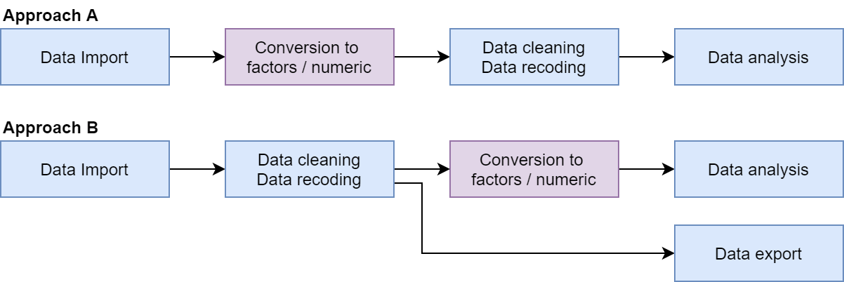
My main interest with Experiment 1.4 is to prepare and/or use the labelled data to work with R. There are principal two approaches:
Procedure 1.4 : Two different procedures to work in R with labelled data
Approach A
In approach A,
haven_labelledvectors are converted into factors or into numeric/character vectors just after data import, usingunlabelled(),to_factor()orunclass(). Then, data cleaning, recoding and analysis are performed using classic R vector types.
Approach B
In approach B,
haven_labelledvectors are kept for data cleaning and coding, allowing to preserved original recoding, in particular if data should be reexported after that step. Functions provided by labelled will be useful for managing value labels. However, as in approach A,haven_labelledvectors will have to be converted into classic factors or numeric vectors before data analysis (in particular modeling) as this is the way categorical and continuous variables should be coded for analysis functions. (Introduction to labelled)
Experiment 1.4 : Inspecting labelled data
R Code 1.35 : Get variable labels of a labelled data frame
labelled::var_label(gss_2016_gssr) #> $age
#> [1] "age of respondent"
#>
#> $grass
#> [1] "should marijuana be made legal"labelled::var_label() to get variables labels of a data frame
The labels of the two variable specifies in more detail their content. For the grass variable we get the question asked in the survey. This is very helpful and saves consulting the codebook.
I am using here the short form with labelled::var_label() but there exist also with labelled::get_variable_labels() a long form which has with it plural form a more consistent syntax.
R Code 1.36 : Get value labels of data frame variables
labelled::val_labels(gss_2016_gssr)#> $age
#> 89 or older don't know
#> 89 NA
#> iap I don't have a job
#> NA NA
#> dk, na, iap no answer
#> NA NA
#> not imputable not imputable
#> NA NA
#> refused skipped on web
#> NA NA
#> uncodeable not available in this release
#> NA NA
#> not available in this year see codebook
#> NA NA
#>
#> $grass
#> should be legal should not be legal
#> 1 2
#> don't know iap
#> NA NA
#> I don't have a job dk, na, iap
#> NA NA
#> no answer not imputable
#> NA NA
#> not imputable refused
#> NA NA
#> skipped on web uncodeable
#> NA NA
#> not available in this release not available in this year
#> NA NA
#> see codebook
#> NAlabelled::val_labels() to get value labels of data frame variables
Important is the start of the list of value labels.
89 of variable age includes values of 89 and older. This is important for the analysis and saves the work of recoding as done in
grass variable we learn that 1 stands for the opinion that Marijuana “should be legal” and two for the opposite.What follows is a comprehensive list of NA values used in the survey, even if many of these values are not used for the two variables considered here.
We know from R Code 1.31 that the grass variable has 1024 NA’s, but we do not know their composition of different NA values. See Listing / Output 1.19 how to get this information.
WATCH OUT! Inconsistency in the function names
There is an inconsistency in the singular vs. plural form between labelled::var_label() and labelled::val_labels(). Both functions show a list of values (= plural) if there are more than one label available.
For value labels exist also a singular version with labelled::val_label() to get a specific value label of a variable.
R Code 1.37 : Using utils::head() on a labelled variable after {labelled} is loaded
## {**labelled**} is loaded through a call in the previous chunk
utils::head(gss_2016_gssr$grass, 10)#> <labelled<double>[10]>: should marijuana be made legal
#> [1] NA(i) 1 2 NA(i) 1 1 NA(i) 2 NA(i) 2
#>
#> Labels:
#> value label
#> 1 should be legal
#> 2 should not be legal
#> NA(d) don't know
#> NA(i) iap
#> NA(j) I don't have a job
#> NA(m) dk, na, iap
#> NA(n) no answer
#> NA(p) not imputable
#> NA(q) not imputable
#> NA(r) refused
#> NA(s) skipped on web
#> NA(u) uncodeable
#> NA(x) not available in this release
#> NA(y) not available in this year
#> NA(z) see codebookUsing utils::head() on a variable when {labelled} is loaded prints a nicely formatted summary of the attached metadata, excluding formats. It shows all NA value labels in the data frame used in the survey, even only some of them is used here. (See Listing / Output 1.19 to get type of NA’s used for a variable.)
We see in the first 10 records of the variable grass
1 (“should be legal”)2 (“should not be legal”) andNA(i) (“iap”)Until now it is not clear what “iap” for the NA(i) type means. If we want download (STATA) files directly from the GSS website we see on the right side a note about the most important NA types. It explains the the abbreviation “iap” stands for “inapplicable”.
Two different meanings of “NA”
With the NA(n) type of missing value “NA” does not mean “Not Applicable” but “No answer”.
Returning only the NA(i) type of a missing value does not mean that there aren’t any other NA types in the data. (See Listing / Output 1.18 to get the types of tagged NA’s of a variable.)
This formatted result of labelled data is better readable as with Listing / Output 1.17, because category and value are in the same line. Compare the result of this code ({labelled} is loaded) with Listing / Output 1.14 ({labelled} is not loaded).
haven::print_labels() as equivalent of head() with {labelled} loaded
With the exception of the specified rows in the head() function, you can get the same nicely formatted list of NA types with haven::print_labels(). (See next tab “Print labels”.)
R Code 1.38 : Print labels
haven::print_labels(gss_2016_gssr$grass)#>
#> Labels:
#> value label
#> 1 should be legal
#> 2 should not be legal
#> NA(d) don't know
#> NA(i) iap
#> NA(j) I don't have a job
#> NA(m) dk, na, iap
#> NA(n) no answer
#> NA(p) not imputable
#> NA(q) not imputable
#> NA(r) refused
#> NA(s) skipped on web
#> NA(u) uncodeable
#> NA(x) not available in this release
#> NA(y) not available in this year
#> NA(z) see codebookFor a detailed explication see previous tab “head()”.
R Code 1.39 : Print unique tagged NA’s
labelled::unique_tagged_na(gss_2016_gssr$grass) |>
labelled::sort_tagged_na() |>
haven::print_tagged_na()#> [1] 1 2 NA(d) NA(i) NA(n)We see that variable grass has three types of NA’s:
NA(d): Don’t know. NA(i): Inapplicable, e.g., these respondents were not asked the marijuana question. NA(n): No answer
Here I have used haven::print_tagged_na() to format tagged NA’s as NA(a), NA(b), etc. (See “Tagged” missing values)
It would be interesting to know the composition of these different NA types. One could reason that there is a big difference between “question not asked” and “no answer”. (See Listing / Output 1.19 to get the composition of the NA types.)
R Code 1.40 : Get the composition of the different types of tagged NA’s
We already know from Listing / Output 1.15 that the variable grass has 1024 NA’s. Now we know also the type composition of these NA’s.
I could not find a similar function in {labelled}, so I have used here haven::na_tag().
There are two ways to work with labelled data in R:
The goal of haven is not to provide a labelled vector that you can use everywhere in your analysis. The goal is to provide an intermediate datastructure that you can convert into a regular R data frame. You can do this by either converting to a factor or stripping the labels ({Haven} vignette Conversion semantics)
Experiment 1.5 : How to convert labelled data for data analysis in R
The second variable grass is the labelled original variable. The third variable (last column to the right) is the modified grass variable.
R Code 1.41 : Convert labelled vectors to factors
#> # A tibble: 10 × 3
#> obs grass grass_factor
#> <int> <dbl+lbl> <fct>
#> 1 1 NA(i) [iap] iap
#> 2 634 NA(i) [iap] iap
#> 3 1098 1 [should be legal] should be legal
#> 4 1152 1 [should be legal] should be legal
#> 5 1177 NA(i) [iap] iap
#> 6 1252 NA(i) [iap] iap
#> 7 2097 1 [should be legal] should be legal
#> 8 2369 1 [should be legal] should be legal
#> 9 2609 1 [should be legal] should be legal
#> 10 2867 2 [should not be legal] should not be legalHere I am using haven::as_factor(). This function also knows how to re-label missing values.
R Code 1.42 : Remove labels
gss_2016_grass |>
dplyr::mutate(grass_unlabelled = haven::zap_labels(grass)) |>
my_glance_data(N = 8, seed = 42)#> # A tibble: 10 × 3
#> obs grass grass_unlabelled
#> <int> <dbl+lbl> <dbl>
#> 1 1 NA(i) [iap] NA
#> 2 634 NA(i) [iap] NA
#> 3 1098 1 [should be legal] 1
#> 4 1152 1 [should be legal] 1
#> 5 1177 NA(i) [iap] NA
#> 6 1252 NA(i) [iap] NA
#> 7 2097 1 [should be legal] 1
#> 8 2369 1 [should be legal] 1
#> 9 2609 1 [should be legal] 1
#> 10 2867 2 [should not be legal] 2R Code 1.43 : Convert special missings to regular R missings
gss_2016_grass |>
dplyr::mutate(grass_rgular_na = haven::zap_missing(grass)) |>
my_glance_data(N = 8, seed = 42)#> # A tibble: 10 × 3
#> obs grass grass_rgular_na
#> <int> <dbl+lbl> <dbl+lbl>
#> 1 1 NA(i) [iap] NA
#> 2 634 NA(i) [iap] NA
#> 3 1098 1 [should be legal] 1 [should be legal]
#> 4 1152 1 [should be legal] 1 [should be legal]
#> 5 1177 NA(i) [iap] NA
#> 6 1252 NA(i) [iap] NA
#> 7 2097 1 [should be legal] 1 [should be legal]
#> 8 2369 1 [should be legal] 1 [should be legal]
#> 9 2609 1 [should be legal] 1 [should be legal]
#> 10 2867 2 [should not be legal] 2 [should not be legal]R Code 1.44 : Remove variable labels from a data frame
#> [1] "******* Original data frame ********"
#> $age
#> [1] "age of respondent"
#>
#> $grass
#> [1] "should marijuana be made legal"
#>
#> [1] "******* Data frame after variable zapped *******"
#> $age
#> NULL
#>
#> $grass
#> NULLYou can combine all three zap-commands.
Creating tables is an important result of preparing data — the main subject of this section. In my research I came up with eight packages that seems to me the most important ones. What follows is a short introduction into these packages.
Experiment 1.6 : Review table packages: {DT}, {flextable}, {gt}, {gtsummary}, {htmlTable}, {kableExtra}, {tableone}, {xtable}
DT is an abbreviation of ‘DataTables.’ Data objects in R can be rendered as HTML tables using the JavaScript library ‘DataTables’ (typically via R Markdown or Shiny).
This R package provides an enhanced version of data.frames with more options for authors and users:
Authors: DT supports data wrangling beside subsetting rows and selecting columns (e.g., computing on columns, sort, grouping). I am not sure if this is really an advantage because it requires the somewhat complex square brackets notation. Using {dplyr} with other {tidyverse} packages seems — for me at least — easier to use. Users: The really advantage of {DT} in my opinion is that the interface allows users to change values and display formats interactively. There are some option in the standard installations and much more with extensions.
Remark 1.1. My conclusion to {DT}
{DT} is my first choice for interactive data exploring and very useful for Explorative Data Analysis (EDA). I have already some experiences with this package but haven’t use it lastly.
Compared with the other table packages {DT} is not in the same category: The following packages are developed as Display Tables (in contrast to Data Tables. Beside of the interactive use {DT}s are Data Tables.
This package helps you to create reporting table from a data frame easily. You can
It is said that {flextable} — together with the sparsely used {huxtable} — “supports the widest range of output formats … [both] support HTML, \(\LaTeX\), and Office formats, and contain most common table features (e.g., conditional formatting).” (Yihui: R Markdown Coobook)
Remark 1.2. My conclusion to {flextable}
{flextable} seems pretty well suited to create sophisticated tables for publications. It is often especially mentioned for exporting into Word files. Maybe I will look into this package in the near future, but currently my priority is {gtsummary}.
{gt} stands for “grammar of tables”. It aims to do for tables what {ggplot2} did for graphics. (Hadley Wickham on X)
{gt} offers a different and easy-to-use set of functions that helps to build display tables from tabular data. The {gt} philosophy states that a comprehensive collection of table parts can be used to create a broad range of functional tables.
It allows you to compose a table by putting together different parts of the table, such as
Some parts are optional. You can also format numbers and add background shading to cells.
 .
.
At the beginning of the development process {gt} supported only HTML, but now you can also use it for LATEX and RTF outputs.
{gt} is developed by the RStudio/Posit team, that stands not only for high quality but also for {tidyverse} compatibility. It was a little surprise for me that the download statistics does not reflect the normally very high figures of RStudio/Posit products. After trying to work with {gt} I believe I know the reasons:
Remark 1.3. My conclusion to {gt}
I tried to work with {gt} but it is cumbersome. I noticed a bug even following the official online tutorial. Maybe {gt} (together with {gtsummary} is better suited for creating easily complex tables in many formats.
The {gtsummary} package provides an efficient way to create publication-ready analytical and summary tables using the R programming language. {gtsummary} summarizes data sets, regression models, and more, using sensible defaults with highly customizable capabilities.
{gtsummary} “was written to be a companion to the {gt} package from RStudio. But not all output types are supported by the {gt} package. Therefore, [the developers] have made it possible to print {gtsummary} tables with various engines.” (gtsummary + Quarto/R Markdown)
Remark 1.4. My conclusion to {gtsummary}
I have tried out {gtsummary} and I am enthusiastic about it! I wrote an introduction with some examples (Section 1.9.2) Now that I understand how it works I will definitely use it. (By the way: Besides the extensive documentation I found that the most effective introduction for me was watching the Youtube video presentation by the developer Daniel D. Sjoberg).
I found {htmlTable} per accident searching the Internet with “r creating complex table”. This package is not mentioned in the literature I have read so far, but it seems not only able to produce complex tables but is also used quite often. Maybe it is the HTML limitation which reduces it application for Online journals because it requires a separate step to produce \(\LaTeX\) tables ready for printing.
It is a pretty old package (version 1.0 appeared already in 2014) but still currently in active development. The last change today (2024-01-18) was version 2.4.2 from 2023-10-29.
From the package documentation:
Advanced Tables for Markdown/HTML
Tables with state-of-the-art layout elements such as row spanners, column spanners, table spanners, zebra striping, and more. While allowing advanced layout, the underlying css-structure is simple in order to maximize compatibility with common word processors. The package also contains a few text formatting functions that help outputting text compatible with HTML/LaTeX.
Beside the extensive vignette documentation there are also some blog articles:
Remark 1.5. My conclusion to {htmlTable}
{htmlTable} seems an interesting package not only for creating complex tables but also for exporting them into Word. But to learn this package is at the moment not on my task list.
{kableExtra} extends the basic functionality of knitr::kable() tables. Although knitr::kable() is simple by design, it has many features missing which are usually available in other packages. {kableExtra} has filled the gap nicely. One of the best thing about {kableExtra} is that most of its table capabilities work for both HTML and PDF formats.
Remark 1.6. My conclusion to {**kableExtra*}
I have already some experiences with {kableExtra}. I used it quasi as an add-on to knitr::kable() during personal HTML publications (Blog, bookdown, Quarto). I believe that other “Table 1” packages like {gtsummary} or maybe also {tableOne) are better suited for display and publication.
The first time I learned about the existence of {tableone} was in Chapter 2 of Statistics with R. Consulting the online documentation it says:
Creates “Table 1”, i.e., description of baseline patient characteristics, which is essential in every medical research. Supports both continuous and categorical variables, as well as p-values and standardized mean differences. Weighted data are supported via the {survey} package. … Most important functions are
CreateTableOne()andsvyCreateTableOne().
Remark 1.7. My conclusion to {tableone}
The package is completely new for me. I have to check it out to see how and when to use. But my priority now is {gtsummary} because
{xtable} is the oldest package and still the table package most used! From the documentation it is clear that it is very useful for the creation of publication ready tables. But I am little hesitant to learn it, because it is not mentioned in current literature and the last change was in April 2019.
Remark 1.8. My conclusion to {xtable}
Learning {xtable} is not on my agenda: It is not clear for me if {xtable} is still in developments and if it is supporting newer approaches. Learning other table packages, especially {gtsummary} probabily together with {gt} has priority for me.
There are other packages as well. But the above eight packages are a first starting point for everybody to learn creating and displaying sophisticated data tables in R. It is good to know about different packages but lastly one has to decide which one to learn and use in daily practice. At the moment my favorites is {gtsummary}.
Resource 1.4 : Other interesting table packages, but currently not considered for my personal purposes
Just for a possible later reference I will add some other table packages I know of.
{reactable}: reactable() creates a data table from tabular data with sorting and pagination by default. The data table is an HTML widget that can be used in R Markdown documents and Shiny applications or viewed from an R console. It is based on the React Table library and made with reactR. Features are:
{ractablefmtr}: The package improves the appearance and formatting of tables created using the reactable R library. It includes many conditional formatters that are highly customizable and easy to use.
The authors of R Markdown Cookbook (Yihui Xie, Christophe Dervieux, Emily Riederer) mention also several other table packages in the section Other packages for creating tables:
I’m not going to introduce the rest of packages, but will just list them here:
Summary of my table packages review
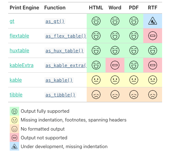
It does not make sense to learn every package. SO I will concentrate on five packages with different usage:
kable() function from {knitr} (see: Section A.43), which is an essential part of the publishing infrastructure for literate programming. It is pretty flexible and could be used in tandem with {gtsummary}.For simple tables one can also use knitr::kable() or just printing the tibble.
As a consequence of my table packages review I experimented with the {gtsummary}. I wanted to create a table where I have information by the variables grass, age in four categories and sex with all their levels in absolute numbers and in percents.
Experiment 1.7 : Experiments with {gtsummary}
grass variable.grass variable.R Code 1.45 : Data used in this {gtsummary} introduction
nhanes_2013_clean <-
    base::readRDS("data/chap01/nhanes_2013_clean.rds")

gtsummary_basic <- nhanes_2013_clean |>

    ## cut age into several defined age groups
    dplyr::mutate(age_cat = base::cut(age,
                   breaks = c(-Inf, 29, 39, 49, 59),
                   labels = c("18 - 29", "30 - 39", "40 - 49", "50 - 59"))) |>
    dplyr::select(-c(nr, age))

save_data_file("chap01", gtsummary_basic, "gtsummary_clean.rds")

base::summary(gtsummary_basic)
#> grass sex age_cat
#> Yes:1991 Male :1792 18 - 29:1154
#> No :1699 Female:1898 30 - 39: 859
#> 40 - 49: 855
#> 50 - 59: 822gtsummary_basic#> # A tibble: 3,690 × 3
#> grass sex age_cat
#> <fct> <fct> <fct>
#> 1 Yes Male 50 - 59
#> 2 Yes Male 50 - 59
#> 3 Yes Female 50 - 59
#> 4 No Female 18 - 29
#> 5 No Female 30 - 39
#> 6 Yes Male 30 - 39
#> 7 No Male 18 - 29
#> 8 Yes Female 30 - 39
#> 9 No Male 50 - 59
#> 10 Yes Male 18 - 29
#> # ℹ 3,680 more rowsI am going to use this dataset to experiment with {gtsummary}.
R Code 1.46 : A very basic summary without any adaptions or modifications
gtsummary_basic <-
    base::readRDS("data/chap01/gtsummary_clean.rds")

gtsummary_basic |>
gtsummary::tbl_summary()| Characteristic | N = 3,6901 |
|---|---|
| grass | 1,991 (54%) |
| sex | |
| Male | 1,792 (49%) |
| Female | 1,898 (51%) |
| age_cat | |
| 18 - 29 | 1,154 (31%) |
| 30 - 39 | 859 (23%) |
| 40 - 49 | 855 (23%) |
| 50 - 59 | 822 (22%) |
| 1 n (%) | |
This is a very basic summary without any adaptions or modifications. It is strange, that there are for grass not separated levels presented. From a video of an introduction to {gtsummary} by the package author Daniel D. Sjoberg I learned that a categorical variable with two levels is interpreted as dichotomous whenever the two levels are labelled 1 and 0, true and false or Yes and No. And dichotomous variable are different as other categorical variables as they are reported by {gtsummary} only with one number (the 1, true or yes value).
Here I am going to change level names of the grass variable to prevent that it is interpreted as a dichotomous variable.
R Code 1.47 : Numbered R Code Title
gtsummary_basic2 <-
    base::readRDS("data/chap01/gtsummary_clean.rds") |>
    dplyr::mutate(grass =
      forcats::fct_recode(grass,
                          "used" = "Yes",
                          "not used" = "No")
            )

gtsummary_basic2 |>
gtsummary::tbl_summary()| Characteristic | N = 3,6901 |
|---|---|
| grass | |
| used | 1,991 (54%) |
| not used | 1,699 (46%) |
| sex | |
| Male | 1,792 (49%) |
| Female | 1,898 (51%) |
| age_cat | |
| 18 - 29 | 1,154 (31%) |
| 30 - 39 | 859 (23%) |
| 40 - 49 | 855 (23%) |
| 50 - 59 | 822 (22%) |
| 1 n (%) | |
This time we can see both levels of grass. But we loose the nice Yes/No answer of the survey.
Another strategy to prevent a dichotomous interpretation is to tell {gtsummary} expressively with the type = argument how a variable has to be interpreted.
R Code 1.48 : Preventing a dichotomous interpretation
gtsummary_basic |>
    gtsummary::tbl_summary(
        type = grass ~ "categorical"
)| Characteristic | N = 3,6901 |
|---|---|
| grass | |
| Yes | 1,991 (54%) |
| No | 1,699 (46%) |
| sex | |
| Male | 1,792 (49%) |
| Female | 1,898 (51%) |
| age_cat | |
| 18 - 29 | 1,154 (31%) |
| 30 - 39 | 859 (23%) |
| 40 - 49 | 855 (23%) |
| 50 - 59 | 822 (22%) |
| 1 n (%) | |
The same output as in the previous tab, but now with the desired Yes/No answer categories.
If there are labelled data {gtsummary} uses them as variable labels. This is a big advantages, especially if the data are already labelled and imported with {haven}. But you can use the {labelled} package to label the variables.
If there are no labelled metadata then the variable name is taken, e.g., in most of the cases you have to provide a better name for the table display.
I am using both methods in the following code chunk: I provided labelled metadata for the grass variable but used new variable names for age_cat and sex.
R Code 1.49 : Changing variable labels
## variant 1 to label variables
# labelled::var_label(
#     gtsummary_basic$grass) <- "Ever used grass or hash?"

## variant 2 to label variables
gtsummary_basic |>
    labelled::set_variable_labels(
        grass = "Ever used grass or hash?"
    ) |>
    gtsummary::tbl_summary(
        # by = grass,
        type = grass ~ "categorical",
        label = list(
            age_cat = "Age Category",
            sex = "Sex"
        )
)| Characteristic | N = 3,6901 |
|---|---|
| Ever used grass or hash? | |
| Yes | 1,991 (54%) |
| No | 1,699 (46%) |
| Sex | |
| Male | 1,792 (49%) |
| Female | 1,898 (51%) |
| Age Category | |
| 18 - 29 | 1,154 (31%) |
| 30 - 39 | 859 (23%) |
| 40 - 49 | 855 (23%) |
| 50 - 59 | 822 (22%) |
| 1 n (%) | |
R Code 1.50 : Summarize data by a grouped variable
gtsummary_group <-  gtsummary_basic |>
    labelled::set_variable_labels(
        grass = "Ever used grass or hash?"
    ) |>
    gtsummary::tbl_summary(
        # by = grass,
        type = grass ~ "categorical",
        label = list(
            age_cat = "Age Category",
            sex = "Sex"
        )
    )

gtsummary_group| Characteristic | N = 3,6901 |
|---|---|
| Ever used grass or hash? | |
| Yes | 1,991 (54%) |
| No | 1,699 (46%) |
| Sex | |
| Male | 1,792 (49%) |
| Female | 1,898 (51%) |
| Age Category | |
| 18 - 29 | 1,154 (31%) |
| 30 - 39 | 859 (23%) |
| 40 - 49 | 855 (23%) |
| 50 - 59 | 822 (22%) |
| 1 n (%) | |
The variable grass is not grouped dplyr::group_by() but inside gtsummary::tbl_summary().
R Code 1.51 : Change table header
gtsummary_group |>
  gtsummary::modify_header(label ~ "**Variable**") |>
  gtsummary::modify_spanning_header(
      gtsummary::show_header_names(gtsummary_group) ~ "**Ever used grass or hash?**")
#> Column Name Header level* N* n* p*
#> label "**Characteristic**" Overall <chr> 3,690 <int> 3,690 <int> 1 <dbl>
#> stat_0 "**N = 3,690**" Overall <chr> 3,690 <int> 3,690 <int> 1 <dbl>#> * These values may be dynamically placed into headers (and other locations).
#> ℹ Review the `modify_header()` (`?gtsummary::modify()`) help for examples.| Variable | N = 3,6901 |
|---|---|
| Ever used grass or hash? | |
| Yes | 1,991 (54%) |
| No | 1,699 (46%) |
| Sex | |
| Male | 1,792 (49%) |
| Female | 1,898 (51%) |
| Age Category | |
| 18 - 29 | 1,154 (31%) |
| 30 - 39 | 859 (23%) |
| 40 - 49 | 855 (23%) |
| 50 - 59 | 822 (22%) |
| 1 n (%) | |
R Code 1.52 : Prepare cross tables and stack them
gtsummary_basic <-
    base::readRDS("data/chap01/gtsummary_clean.rds")

gtsummary_cross1 <- gtsummary_basic |>
    labelled::set_variable_labels(
            grass = "**Ever used grass or hash?**"
        ) |>
    gtsummary::tbl_cross(
        label = list(
            age_cat = "Age Category",
            sex = "Sex"
        ),
        row = age_cat,
        col = grass,
        percent = "cell"
    ) |>
    gtsummary::modify_header(
      stat_1 = '**Yes**',
      stat_2 = '**No**',
      stat_0 = '**Total**'
    )

gtsummary_cross2 <- gtsummary_basic |>
    labelled::set_variable_labels(
            grass = "**Ever used grass or hash?**"
        ) |>
    gtsummary::tbl_cross(
        label = list(
            age_cat = "Age Category",
            sex = "Sex"
        ),
        row = sex,
        col = grass,
        percent = "cell"
    ) |>
    gtsummary::modify_header(
      stat_1 = '**Yes**',
      stat_2 = '**No**',
      stat_0 = '**Total**'
    )

gtsummary::tbl_stack(
    list(gtsummary_cross1,
         gtsummary_cross2)
    ) |>
    gtsummary::bold_labels()
Ever used grass or hash?
|
Total | ||
|---|---|---|---|
| Yes | No | ||
| Age Category | |||
| 18 - 29 | 662 (18%) | 492 (13%) | 1,154 (31%) |
| 30 - 39 | 466 (13%) | 393 (11%) | 859 (23%) |
| 40 - 49 | 405 (11%) | 450 (12%) | 855 (23%) |
| 50 - 59 | 458 (12%) | 364 (9.9%) | 822 (22%) |
| Total | 1,991 (54%) | 1,699 (46%) | 3,690 (100%) |
| Sex | |||
| Male | 1,072 (29%) | 720 (20%) | 1,792 (49%) |
| Female | 919 (25%) | 979 (27%) | 1,898 (51%) |
| Total | 1,991 (54%) | 1,699 (46%) | 3,690 (100%) |
R Code 1.53 : Stratify tables
gtsummary_basic <-
    base::readRDS("data/chap01/gtsummary_clean.rds")

gtsummary_basic |>
    gtsummary::tbl_strata(
        strata = grass,
        ~ .x |>
    gtsummary::tbl_summary(
        by = sex,
        label = age_cat ~ "Age Category"
        ) |>
    gtsummary::add_overall() |>
    gtsummary::modify_header(
        label = "**Variables**",
        gtsummary::all_stat_cols() ~ "**{level}**"
        )
    ) |>
gtsummary::bold_labels() | Variables |
Yes
|
No
|
||||
|---|---|---|---|---|---|---|
| Overall1 | Male1 | Female1 | Overall1 | Male1 | Female1 | |
| Age Category | ||||||
| 18 - 29 | 662 (33%) | 360 (34%) | 302 (33%) | 492 (29%) | 208 (29%) | 284 (29%) |
| 30 - 39 | 466 (23%) | 267 (25%) | 199 (22%) | 393 (23%) | 163 (23%) | 230 (23%) |
| 40 - 49 | 405 (20%) | 202 (19%) | 203 (22%) | 450 (26%) | 198 (28%) | 252 (26%) |
| 50 - 59 | 458 (23%) | 243 (23%) | 215 (23%) | 364 (21%) | 151 (21%) | 213 (22%) |
| 1 n (%) | ||||||
Experiment 1.8 : Developing a graph showing the timeline of respondents opinion about legalizing marijuana (1973-2022)
R Code 1.54 : Load the GSS data from 1972-2022 and select appropriate variables
(This R code chunk has no visible output)
R Code 1.55 : Clean grass-legal dataset
## run only once (manually) ##########
gss_grass_legal <-
    base::readRDS("data/chap01/gss_grass_legal.rds")

gss_grass_legal_clean <- gss_grass_legal |>
    tidyr::drop_na() |>
    dplyr::mutate(
        grass = forcats::as_factor(grass),
        grass = forcats::fct_drop(grass),
        year = base::as.numeric(year),
        age = base::as.numeric(age)
    )

save_data_file("chap01", gss_grass_legal_clean, "gss_grass_legal_clean.rds")(This R code chunk has no visible output)
R Code 1.56 : Show summary of cleaned dataset
grass_legal <-
    base::readRDS("data/chap01/gss_grass_legal_clean.rds")

## remove comma from big numbers
gtsummary::theme_gtsummary_language("en", big.mark = "")


grass_legal |>
  gtsummary::tbl_summary(
    label = list(
        year ~ "Year",
        age ~ "Age",
        grass ~ "Should marijuana be legal?"
    ),
    type = list(age ~ "continuous2", year ~ "continuous2"),
    statistic =
         list(
            age ~ c(
      "{mean} ({sd})",
      "{median} ({p25}, {p75})",
      "{min}, {max}"
         ),
            year ~ c("{min}, {max}")
    )
  ) |>
  gtsummary::italicize_levels() |>
gtsummary::bold_labels()| Characteristic | N = 384791 |
|---|---|
| Year | |
| Min, Max | 1973, 2022 |
| Age | |
| Mean (SD) | 46 (18) |
| Median (Q1, Q3) | 43 (31, 59) |
| Min, Max | 18, 89 |
| Should marijuana be legal? | |
| should be legal | 12589 (33%) |
| should not be legal | 25890 (67%) |
| 1 n (%) | |
WATCH OUT! Summary with labelled data
I used for the summary the labelled data from the {gssr} package. This has the big advantage that I didn’t recode the variable names and could use the variable and value metadata!
But {gtsummary} warned me to see that this is only “an intermediate data structure not meant for analysis”.
Column(s) age are class “haven_labelled”. This is an intermediate datastructure not meant for analysis. Convert columns with
haven::as_factor(),labelled::to_factor(),labelled::unlabelled(), andunclass(). “haven_labelled” value labels are ignored when columns are not converted. Failure to convert may have unintended consequences or result in error.
R Code 1.57 : Prepare data for timeline graph
(This R code chunk has no visible output)
R Code 1.58 : Timeline of respondents opinion about legalizing marijuana (1973-2022)
grass_legal2 |>
    # dplyr::group_by(year) |>
    ggplot2::ggplot(ggplot2::aes(
        x = year,
        y = perc,
        color = grass)) +
    ggplot2::geom_point() +
    ggplot2::theme_bw() +
    ggplot2::scale_color_manual(
        values = c("#79a778", '#7662aa')
        ) +
    ggplot2::scale_x_continuous(
        breaks = c(1973, seq(1978, 2022, 4), 2022)
        ) +
    ggplot2::theme(axis.text.x =
          ggplot2::element_text(angle = 45, vjust = 0.5)) +
    ggplot2::labs(
        x = "Should marijuana be legal?",
        y = "Percent of responses",
        color = "Marijuana") +
    ggplot2::theme(legend.position = c(.82, .85))
#> Warning: A numeric `legend.position` argument in `theme()` was deprecated in ggplot2
#> 3.5.0.
#> ℹ Please use the `legend.position.inside` argument of `theme()` instead.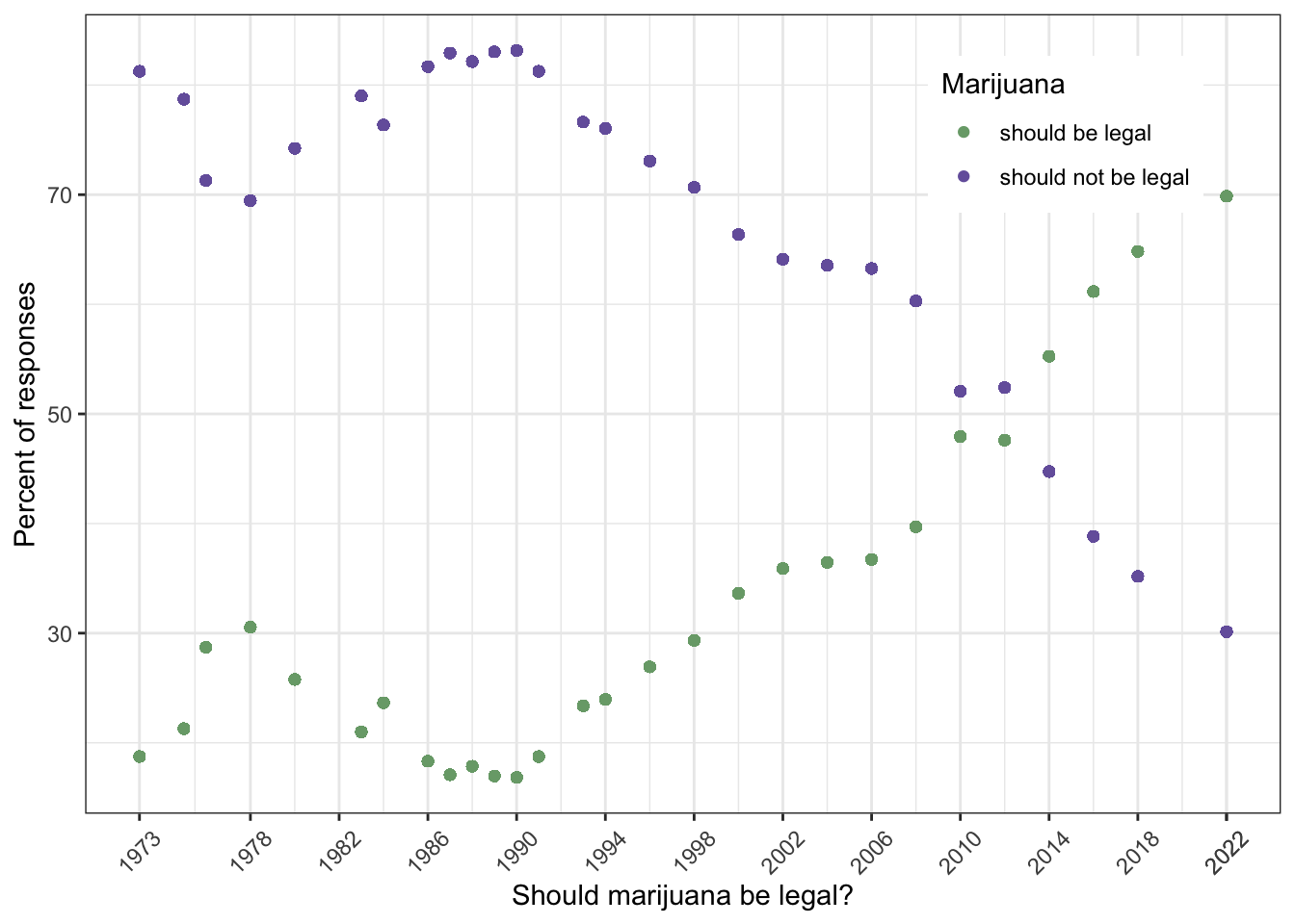
Graph 1.12 shows that the proportion of people that support legalizing marijuana is (with the exception of 1978-1990) continuously rising. Starting from 19% support in 1973 approval hits 70% in 2022, the last date where data are available. The turning point where the proportion of affirmation was the first time greater than the disapproval was in 2014 (55/45).
| term | definition |
|---|---|
| ACSPRI | Australian Consortium for Social and Political Research Inc. oganizes conferences and delivers course. (<a href="https://www.acspri.org.au/">ACSPRI</a>) |
| CSV | Text files where the values are separated with commas (Comma Separated Values = CSV). These files have the file extension .csv |
| Data Tables | Data Tables are --- in contrast to Display Tables --- for analysis and not for presentation. Another purpose of Data Tables is to store, retrieve and share information digitally. In R they are tibbles, data.frames etc. |
| Display Tables | Display Tables are in constrast to Data Tables. You would find them in a web page, a journal article, or in a magazine. Such tables are for presentation, often to facilitate the construction of “Table 1”, i.e., baseline characteristics table commonly found in research papers. (<a href= "https://gt.rstudio.com/articles/gt.html">Introduction to Creating gt Tables</a>) |
| EDA | Explorative Data Analysis is an approach of analyzing data sets to summarize their main characteristics, often using statistical graphics and other data visualization methods. A statistical model can be used or not, but primarily EDA is for seeing what the data can tell us beyond the formal modeling and thereby contrasts traditional hypothesis testing. (<a href="https://en.wikipedia.org/wiki/Exploratory_data_analysis">Wikipedia</a>) |
| General Social Survey | A large survey of a sample of people in the United States conducted regularly since 1972; the General Social Survey is abbreviated GSS and is conducted by the National Opinion Research Center at the University of Chicago. (Harris, Glossary) |
| GSS | A large survey of a sample of people in the United States conducted regularly since 1972; the General Social Survey is abbreviated GSS and is conducted by the National Opinion Research Center at the University of Chicago. (Harris, Glossary) |
| Literate Programming | Literate programming is a methodology that combines a programming language with a documentation language, thereby making programs more robust, more portable, more easily maintained, and arguably more fun to write than programs that are written only in a high-level language. The main idea is to treat a program as a piece of literature, addressed to human beings rather than to a computer.(<a href="https://www-cs-faculty.stanford.edu/~knuth/lp.html">Donald Knuth</a>) |
| Microdata | Microdata are unit-level data obtained from sample surveys, censuses, and administrative systems. They provide information about characteristics of individual people or entities such as households, business enterprises, facilities, farms or even geographical areas such as villages or towns. They allow in-depth understanding of socio-economic issues by studying relationships and interactions among phenomena. Microdata are thus key to designing projects and formulating policies, targeting interventions and monitoring and measuring the impact and results of projects, interventions and policies. ([The World Bank] |
| NHANES | The National Health and Nutrition Examination Survey (NHANES) is a program of studies designed to assess the health and nutritional status of adults and children in the United States. The survey is unique in that it combines interviews and physical examinations. (<a href="https://www.cdc.gov/nchs/nhanes/about_nhanes.htm">NHANES</a>) |
| Prolog | A set of comments at the top of a code file that provides information about what is in the file (SwR, Glossary) |
| Table 1 | Descriptive statistics are often displayed in the first table in a published article or report and are therefore often called <i>Table 1 statistics</i> or the <i>descriptives</i>. (SwR) |
Session Info
sessioninfo::session_info()#> ─ Session info ───────────────────────────────────────────────────────────────
#> setting value
#> version R version 4.4.2 (2024-10-31)
#> os macOS Sequoia 15.1
#> system x86_64, darwin20
#> ui X11
#> language (EN)
#> collate en_US.UTF-8
#> ctype en_US.UTF-8
#> tz Europe/Vienna
#> date 2024-11-13
#> pandoc 3.5 @ /usr/local/bin/ (via rmarkdown)
#>
#> ─ Packages ───────────────────────────────────────────────────────────────────
#> package * version date (UTC) lib source
#> base64enc 0.1-3 2015-07-28 [2] CRAN (R 4.4.0)
#> bit 4.5.0 2024-09-20 [2] CRAN (R 4.4.1)
#> bit64 4.5.2 2024-09-22 [2] CRAN (R 4.4.1)
#> cards 0.3.0 2024-10-03 [2] CRAN (R 4.4.1)
#> cli 3.6.3 2024-06-21 [2] CRAN (R 4.4.1)
#> codetools 0.2-20 2024-03-31 [2] CRAN (R 4.4.2)
#> colorspace 2.1-1 2024-07-26 [2] CRAN (R 4.4.0)
#> commonmark 1.9.2 2024-10-04 [2] CRAN (R 4.4.1)
#> crayon 1.5.3 2024-06-20 [2] CRAN (R 4.4.0)
#> curl 6.0.0 2024-11-05 [2] CRAN (R 4.4.1)
#> digest 0.6.37 2024-08-19 [2] CRAN (R 4.4.1)
#> dplyr 1.1.4 2023-11-17 [2] CRAN (R 4.4.0)
#> evaluate 1.0.1 2024-10-10 [2] CRAN (R 4.4.1)
#> fansi 1.0.6 2023-12-08 [2] CRAN (R 4.4.0)
#> farver 2.1.2 2024-05-13 [2] CRAN (R 4.4.0)
#> fastmap 1.2.0 2024-05-15 [2] CRAN (R 4.4.0)
#> forcats 1.0.0 2023-01-29 [2] CRAN (R 4.4.0)
#> generics 0.1.3 2022-07-05 [2] CRAN (R 4.4.0)
#> ggplot2 3.5.1 2024-04-23 [2] CRAN (R 4.4.0)
#> glossary * 1.0.0.9003 2024-08-05 [2] Github (debruine/glossary@05e4a61)
#> glue 1.8.0 2024-09-30 [2] CRAN (R 4.4.1)
#> gt 0.11.1 2024-10-04 [2] CRAN (R 4.4.1)
#> gtable 0.3.6 2024-10-25 [2] CRAN (R 4.4.1)
#> gtsummary 2.0.3 2024-10-04 [2] CRAN (R 4.4.1)
#> haven 2.5.4 2023-11-30 [2] CRAN (R 4.4.0)
#> here 1.0.1 2020-12-13 [2] CRAN (R 4.4.0)
#> hms 1.1.3 2023-03-21 [2] CRAN (R 4.4.0)
#> htmltools 0.5.8.1 2024-04-04 [2] CRAN (R 4.4.0)
#> htmlwidgets 1.6.4 2023-12-06 [2] CRAN (R 4.4.0)
#> jsonlite 1.8.9 2024-09-20 [2] CRAN (R 4.4.1)
#> kableExtra 1.4.0 2024-01-24 [2] CRAN (R 4.4.0)
#> knitr 1.49 2024-11-08 [2] CRAN (R 4.4.1)
#> labeling 0.4.3 2023-08-29 [2] CRAN (R 4.4.0)
#> labelled 2.13.0 2024-04-23 [2] CRAN (R 4.4.0)
#> lifecycle 1.0.4 2023-11-07 [2] CRAN (R 4.4.0)
#> magrittr 2.0.3 2022-03-30 [2] CRAN (R 4.4.0)
#> markdown 1.13 2024-06-04 [2] CRAN (R 4.4.0)
#> munsell 0.5.1 2024-04-01 [2] CRAN (R 4.4.0)
#> pillar 1.9.0 2023-03-22 [2] CRAN (R 4.4.0)
#> pkgconfig 2.0.3 2019-09-22 [2] CRAN (R 4.4.0)
#> purrr 1.0.2 2023-08-10 [2] CRAN (R 4.4.0)
#> R6 2.5.1 2021-08-19 [2] CRAN (R 4.4.0)
#> readr 2.1.5 2024-01-10 [2] CRAN (R 4.4.0)
#> repr 1.1.7 2024-03-22 [2] CRAN (R 4.4.0)
#> rlang 1.1.4 2024-06-04 [2] CRAN (R 4.4.0)
#> rmarkdown 2.29 2024-11-04 [2] CRAN (R 4.4.1)
#> rprojroot 2.0.4 2023-11-05 [2] CRAN (R 4.4.0)
#> rstudioapi 0.17.1 2024-10-22 [2] CRAN (R 4.4.1)
#> rversions 2.1.2 2022-08-31 [2] CRAN (R 4.4.0)
#> sass 0.4.9 2024-03-15 [2] CRAN (R 4.4.0)
#> scales 1.3.0 2023-11-28 [2] CRAN (R 4.4.0)
#> sessioninfo 1.2.2 2021-12-06 [2] CRAN (R 4.4.0)
#> skimr 2.1.5 2022-12-23 [2] CRAN (R 4.4.0)
#> stringi 1.8.4 2024-05-06 [2] CRAN (R 4.4.0)
#> stringr 1.5.1 2023-11-14 [2] CRAN (R 4.4.0)
#> svglite 2.1.3 2023-12-08 [2] CRAN (R 4.4.0)
#> systemfonts 1.1.0 2024-05-15 [2] CRAN (R 4.4.0)
#> tibble 3.2.1 2023-03-20 [2] CRAN (R 4.4.0)
#> tidyr 1.3.1 2024-01-24 [2] CRAN (R 4.4.0)
#> tidyselect 1.2.1 2024-03-11 [2] CRAN (R 4.4.0)
#> tzdb 0.4.0 2023-05-12 [2] CRAN (R 4.4.0)
#> utf8 1.2.4 2023-10-22 [2] CRAN (R 4.4.0)
#> vctrs 0.6.5 2023-12-01 [2] CRAN (R 4.4.0)
#> viridisLite 0.4.2 2023-05-02 [2] CRAN (R 4.4.0)
#> vroom 1.6.5 2023-12-05 [2] CRAN (R 4.4.0)
#> withr 3.0.2 2024-10-28 [2] CRAN (R 4.4.1)
#> xfun 0.49 2024-10-31 [2] CRAN (R 4.4.1)
#> xml2 1.3.6 2023-12-04 [2] CRAN (R 4.4.0)
#> yaml 2.3.10 2024-07-26 [2] CRAN (R 4.4.0)
#>
#> [1] /Library/Frameworks/R.framework/Versions/4.4-x86_64/library
#> [2] /Library/Frameworks/R.framework/Versions/4.4-x86_64/Resources/library
#>
#> ──────────────────────────────────────────────────────────────────────────────To prevent conflict with the labelled class from the {Hmisc} package {haven} has changed with version 2.0.0 its label class names from labelled and labelled_spss to haven_labelled and haven_labelled_spss. (See GitHub Issue #329.)↩︎