Code
## run only once (manually)
## load "GSS" data.frame into memory
base::load("data/chap07/gss2018.rda")

gss_2018 <- GSS
save_data_file("chap07", gss_2018, "gss_2018.rds")Objectives for chapter 07
SwR Achievements
ANOVA is the statistical method used for comparing means across three or more groups.
Resource 7.1 : Data, codebook, and R packages for learning about descriptive statistics
Data
Two options:
gss2018.rda data set from https://edge.sagepub.com/harris1e.(As a direct download with the {gssr} package results in labelled data with different column names and the necessary transformation will not gain any additional knowledge for me, I will take the gss2018.rda data set from the book.)
Codebook
Two options:
Packages
R Code 7.1 : Get book GSS data set gss2018.rda and save it as gss_2018.rds
## run only once (manually)
## load "GSS" data.frame into memory
base::load("data/chap07/gss2018.rda")
gss_2018 <- GSS
save_data_file("chap07", gss_2018, "gss_2018.rds")(For this R code chunk is no output available)
R Code 7.2 : Show summary for some gss_2018 data
#>     USETECH           HAPPY            SEX             AGE
#>  Min.   : -1.00   Min.   :1.000   Min.   :1.000   Min.   :18.00
#>  1st Qu.: -1.00   1st Qu.:1.000   1st Qu.:1.000   1st Qu.:34.00
#>  Median : 10.00   Median :2.000   Median :2.000   Median :48.00
#>  Mean   : 48.09   Mean   :1.855   Mean   :1.552   Mean   :49.13
#>  3rd Qu.: 80.00   3rd Qu.:2.000   3rd Qu.:2.000   3rd Qu.:63.00
#>  Max.   :999.00   Max.   :8.000   Max.   :2.000   Max.   :99.00
#>      DEGREE
#>  Min.   :0.000
#>  1st Qu.:1.000
#>  Median :1.000
#>  Mean   :1.684
#>  3rd Qu.:3.000
#> Max. :4.000Procedure 7.1 : To get the full information for a variable in GSS
> symbol or by pressing the “Show Expanded View”-button.
Recoding data exactly as in the book
As we are going to use the data set from the book and not the current data set as it is today (2024-03-25) saved at the GSS website, we will for instance USETECH recode -1, 998 and 999 as missing data in our data frame (and not the current values).
Generally: There is nothing new for me in recoding the data. So I will apply all the necessary recoding in the next subsection in only one R code chunk.
R Code 7.3 : Clean gss_2018 data
## run only once (manually) ############
gss_2018 <- base::readRDS("data/chap07/gss_2018.rds")

gss_2018_clean <- gss_2018 |>
    dplyr::select(c("USETECH", "HAPPY", "SEX", "AGE", "DEGREE")) |>
    dplyr::mutate(USETECH = dplyr::na_if(x = USETECH, y = -1)) |>
    dplyr::mutate(USETECH = dplyr::na_if(x = USETECH, y = 998)) |>
    dplyr::mutate(USETECH = dplyr::na_if(x = USETECH, y = 999)) |>
    dplyr::mutate(AGE = dplyr::na_if(x = AGE, y = 98)) |>
    dplyr::mutate(AGE = dplyr::na_if(x = AGE, y = 99)) |>
    dplyr::mutate(DEGREE = dplyr::na_if(x = DEGREE, y = 8)) |>
    dplyr::mutate(DEGREE = dplyr::na_if(x = DEGREE, y = 9)) |>
    dplyr::mutate(HAPPY = dplyr::na_if(x = HAPPY, y = 8)) |>
    dplyr::mutate(HAPPY = dplyr::na_if(x = HAPPY, y = 9)) |>
    dplyr::mutate(HAPPY = dplyr::na_if(x = HAPPY, y = 0)) |>

    dplyr::mutate(SEX = forcats::as_factor(SEX)) |>
    dplyr::mutate(DEGREE = forcats::as_factor(DEGREE)) |>
    dplyr::mutate(HAPPY = forcats::as_factor(HAPPY)) |>

    dplyr::mutate(SEX = forcats::fct_recode(SEX,
                                            male = "1",
                                            female = "2")) |>
    dplyr::mutate(DEGREE = forcats::fct_recode(DEGREE,
                                            "< high school" = "0",
                                            "high school" = "1",
                                            "junior college" = "2",
                                            "bachelor" = "3",
                                            "graduate" = "4")) |>
    dplyr::mutate(HAPPY = forcats::fct_recode(HAPPY,
                                        "very happy" = "1",
                                        "pretty happy" = "2",
                                        "not too happy" = "3"))

save_data_file("chap07", gss_2018_clean, "gss_2018_clean.rds")

base::summary(gss_2018_clean)
#> USETECH HAPPY SEX AGE
#> Min. : 0.00 very happy : 701 male :1051 Min. :18.00
#> 1st Qu.: 15.00 pretty happy :1304 female:1294 1st Qu.:34.00
#> Median : 60.00 not too happy: 336 Median :48.00
#> Mean : 55.15 NA's : 4 Mean :48.98
#> 3rd Qu.: 90.00 3rd Qu.:63.00
#> Max. :100.00 Max. :89.00
#> NA's :936 NA's :7
#> DEGREE
#> < high school : 262
#> high school :1175
#> junior college: 196
#> bachelor : 465
#> graduate : 247
#>
#> The work in this section is done in Section 7.3.2, Section 7.3.3 and Section 7.3.4.
Question to explore: Do people with higher educational degrees use technology at work more than people with lower degree?
Example 7.1 : Explorative Data Analysis (EDA)
R Code 7.4 : Mean and standard deviation of technology use by respondent’s highest degree
#> # A tibble: 5 × 3
#>   DEGREE         mean_usetech sd_usetech
#>   <fct>                 <dbl>      <dbl>
#> 1 < high school          24.8       36.2
#> 2 high school            49.6       38.6
#> 3 junior college         62.4       35.2
#> 4 bachelor               67.9       32.1
#> 5 graduate               68.7       30.2
It seems that we could affirm our question. With higher degree the value of the mean (representing the percentage of technology usage) is rising. But we have a big standard deviation, especially in the lowest degree group (\(sd \approx 1.5 mean\)). This could indicate that we have not a normal distribution because of high kurtosis, e.g. we could have more observations in the tails than a normal distribution would have (platykurtic).
R Code 7.5 : Distribution of work time spent using technology by educational attainment
gg_gss_2018 <- gss_2018_clean |>
  tidyr::drop_na(USETECH) |>
  ggplot2::ggplot(
      ggplot2::aes(
          x = DEGREE,
          y = USETECH
          )
      ) +
  ggplot2::geom_jitter(
      ggplot2::aes(color = DEGREE), alpha = .6
      ) +
  ggplot2::geom_boxplot(
      ggplot2::aes(fill = DEGREE), alpha = .4
      ) +
  ggplot2::scale_fill_brewer(
      palette = "Spectral",
      guide = "none"
      ) +
  ggplot2::scale_color_brewer(
      palette = "Spectral",
      guide = "none") +
  ggplot2::theme_bw() +
  ggplot2::labs(
      x = "Highest educational attainment",
      y = "Percent of time spent using technology"
      )

gg_gss_2018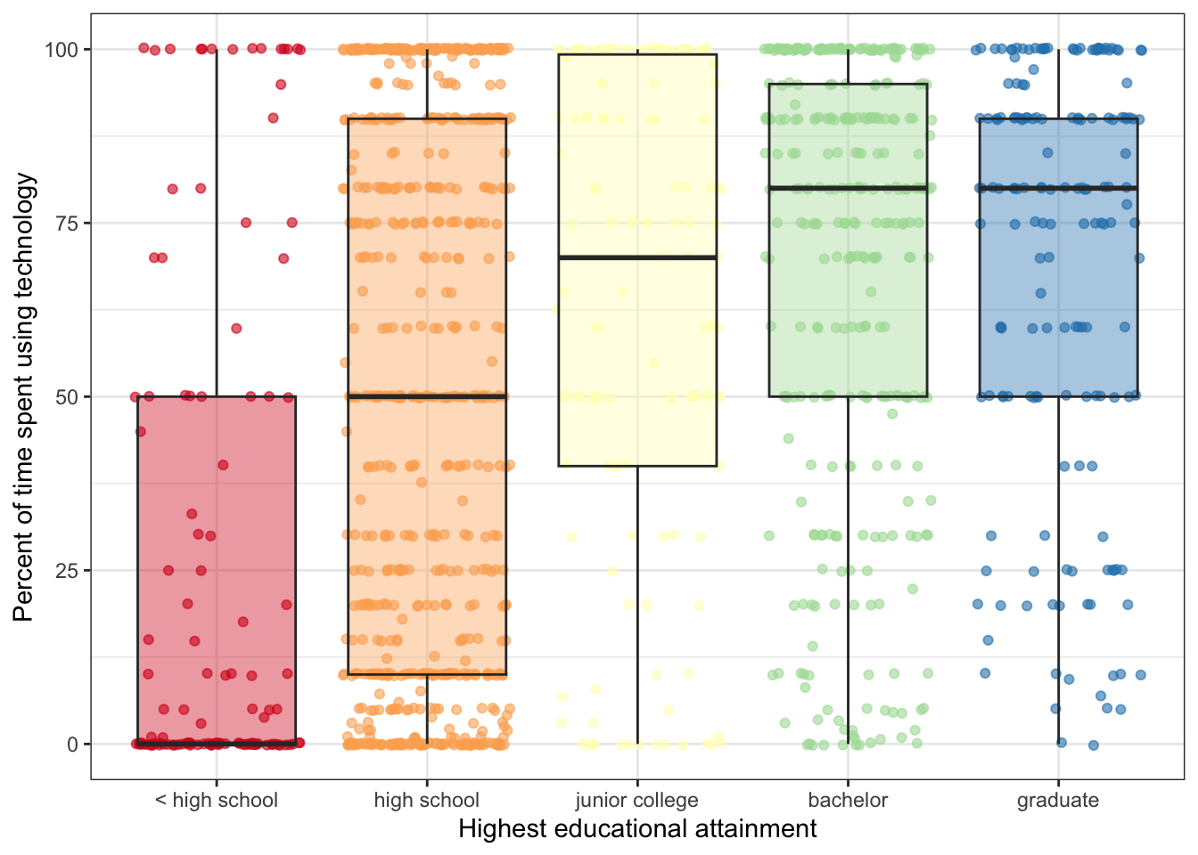
Harris uses with this graph (Figure 7.4 in her book) the color schemes from ColorBrewer. See for more details the color palettes of RColorBrewer and the screenshot of the tmaptools::palette_explorer() function.
But the chosen color palette is not appropriate for people with color vision deficiency (CVD). Mainly the yellow color is problematic as can be demonstrated with the following plot as can be seen in the next tab
R Code 7.6 : Distribution of work time spent using technology by educational attainment
colorblindr::cvd_grid(gg_gss_2018, severity = 1)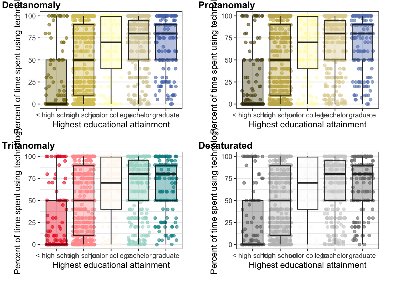
R Code 7.7 : Distribution of work time spent using technology by educational attainment (colorblind save)
gg2_gss_2018 <- gss_2018_clean |>
  tidyr::drop_na(USETECH) |>
  ggplot2::ggplot(
      ggplot2::aes(
          x = DEGREE,
          y = USETECH
          )
      ) +
  ggplot2::geom_jitter(
      ggplot2::aes(color = DEGREE), alpha = .6
      ) +
  ggplot2::geom_boxplot(
      ggplot2::aes(fill = DEGREE), alpha = .4
      ) +
  ggokabeito::scale_color_okabe_ito(guide = "none") +
  ggokabeito::scale_fill_okabe_ito(guide = "none") +
  ggplot2::theme_bw() +
  ggplot2::labs(
      x = "Highest educational attainment",
      y = "Percent of time spent using technology"
  )

gg2_gss_2018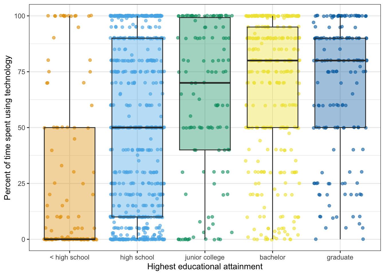
colorblindr::cvd_grid(gg2_gss_2018)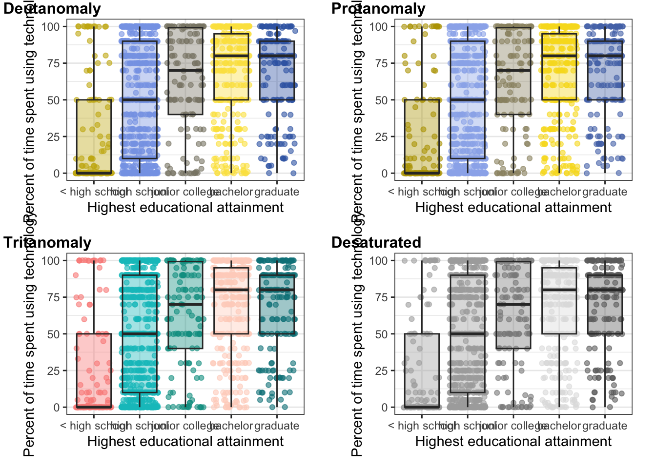
Although the color palette “Okabe-Ito” is also using a kind of yellow the result is much better in all CVD variants. Compare it with Graph 7.3.
What we can see with the graph is that there are many observation at the bottom and at the top of the range of the variable USETECH.
WATCH OUT! ANOVA with floor and ceiling effect
When there are floor or ceiling effects, this often means that the variation in a measure is limited by its range. Since ANOVA is an analysis of variance, which examines central tendency and variation together, the limitations of floor and ceiling effects can result in not finding differences when there are differences.
Sometimes floor or ceiling effects are hints that the range of the variable is not chosen correctly. But this does not apply in our case, because the range of using technology from 0 to 100% is as wide as it can be. Besides I believe these extreme values do not relate to the true value of technology use in work. I think that today there is almost no work without some sort of technology support. On the other hand it is no very likely that 100% (every second of work) of technology use is realistic.
You can’t apply the t-test as a number of different pairwise tests to compare categorical variables that have several levels (groups). The problem is that the Type I error piles ab with several tests. For example: With five groups in the DEGREE variable, pairwise comparisons with a t-test (i.e., conducting pairwise comparisons) would result in 10 t-tests. If each t-test had a p-value threshold of .05 for statistical significance, the probability of at least one Type I error is fairly high.
Formula 7.1 : Probability of a Type I error when there are multiple comparisons
\[ \begin{align*} \alpha_{f} = 1 - (1 - \alpha_{i})^c \\ c = \frac{k(k-1)}{2} \end{align*} \tag{7.1}\]
For a five-group DEGREE variable with \(\alpha = .05\) for each pairwise comparison the familywise \(\alpha_{f}\) would be:
\[ \begin{align*} \alpha_{f} = 1-(1-0.05_{i})^\frac{5(5-1)}{2} = \\ \alpha_{f} = 1-(1-0.05_{i})^{10} = 0.4012631 \end{align*} \]
With 10 pairwise comparisons, the familywise \(\alpha_{f}\) indicated there would be a 40% probability of making a Type I error. To control this error rate, and for efficiency, use a single ANOVA test instead of 10 t-tests. ANOVA is useful for testing whether three or more means are equal. It can be used with two means, but the t-test is preferable because it is more straightforward.
Running many tests
I believe that the problem of a rising Type I error with a growing number of pairwise comparisons is also valid for other type of tests. Each test has the .05 threshold and a collection of many different tests with the same data rises the probability of making a Type I error. Using this strategy consciously is one form of p-hacking.
The F-statistic is a ratio where the variation between the groups is compared to the variation within the groups. The between-group variation is in the numerator to calculate F, while the within-group variation is in the denominator.
Subtracting the grand mean from the group mean results in the difference between the group and the overall sample. The difference between the grand mean and the group mean can be positive or negative and so is squared for the sum to more accurately represent the total of the differences. This squared value is then multiplied by nj or the number of people in the group and divided by k – 1, where k is the number of groups. This results in a numerator that quantifies the difference between the group means and grand mean for all the participants in the sample.
The denominator sums the squared difference between each individual observation yij and the mean of the individual’s group, quantifying how far the individuals in the group are from the mean of the group. This is divided by the number of individuals in the whole sample minus the number of groups.
Formula 7.2 : F-Statistic
\[ \begin{align*} F &= \frac{\text{between-group variability}}{\text{within-group variability}} \\ &= \frac{\text{explained variance}}{\text{unexplained variance}} \\ &= \frac{s_{between}^2}{s_{within}^2} \end{align*} \tag{7.2}\]
The F-statistic, then, could be referred to as a ratio of explained to unexplained variance. That is, how much of the variability in the outcome does the model explain compared to how much it leaves unexplained? The larger the F-statistic, the more the model has explained compared to what it has left unexplained.
The F-statistic can also be represented as the ratio of the variance between the groups to the variance within the groups.
Example 7.2 : F-test for using technology at the work place
R Code 7.8 : Applying F-test stats::oneway.test()
gss_2018_clean <- base::readRDS("data/chap07/gss_2018_clean.rds")

stats::oneway.test(
    formula = USETECH ~ DEGREE,
    data = gss_2018_clean,
    var.equal = TRUE
)#>
#> One-way analysis of means
#>
#> data: USETECH and DEGREE
#> F = 43.304, num df = 4, denom df = 1404, p-value < 2.2e-16R Code 7.9 : Distribution of work time spent using technology by educational attainment, with grand mean and group means (Replication of book Figure 7.5)
grand_mean <-
base::mean(gss_2018_clean$USETECH, na.rm = TRUE)
group_means <- gss_2018_clean |>
tidyr::drop_na(USETECH, DEGREE) |>
dplyr::group_by(DEGREE) |>
dplyr::summarize(mean = mean(USETECH))
gg3_gss_2018 <- gss_2018_clean |>
tidyr::drop_na(USETECH) |>
ggplot2::ggplot(
ggplot2::aes(
x = DEGREE,
y = USETECH
)
) +
ggplot2::geom_jitter(
ggplot2::aes(
alpha = .6
),
color = "darkgrey"
) +
ggplot2::geom_hline(
ggplot2::aes(
yintercept = grand_mean,
linetype = "solid"
),
color = "steelblue",
linewidth = 1
) +
ggplot2::geom_point(
data = group_means,
ggplot2::aes(
x = DEGREE,
y = mean,
size = 3
),
color = "purple4",
inherit.aes = FALSE
) +
ggplot2::theme_bw() +
ggplot2::labs(
x = "Highest educational attainment",
y = "Percent of time spent using technology"
) +
ggplot2::scale_size_continuous(
name = "",
labels = "Group mean"
) +
ggplot2::scale_linetype_discrete(
name = "",
labels = "Grand mean"
) +
ggplot2::scale_alpha_continuous(
name = "",
labels = "Observation"
)
gg3_gss_2018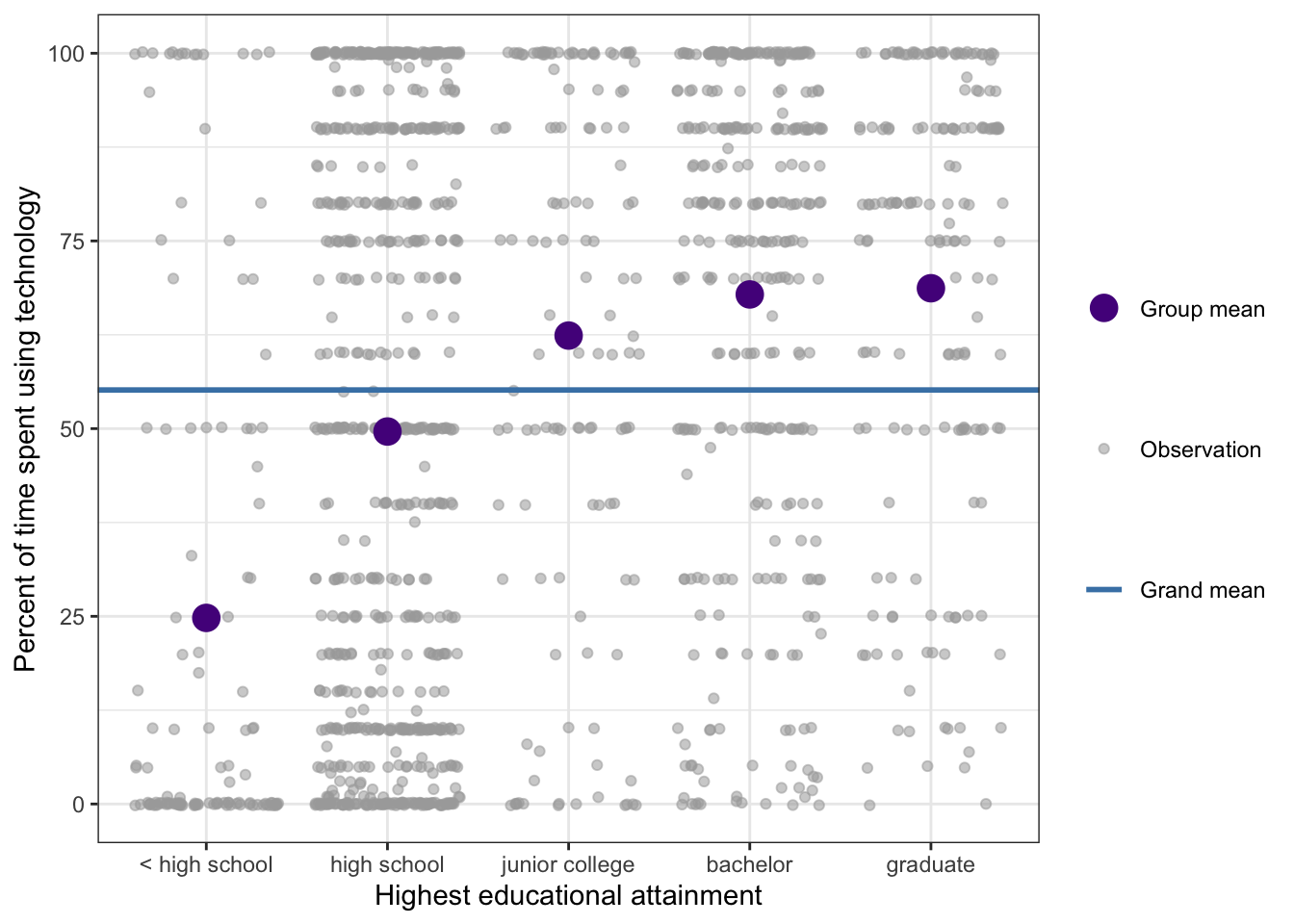
This R-Code junk replicates book’s Figure 7.5, which has no accompanying R code.
For each group, the group mean does a better job than the overall mean of explaining tech use for that group. The difference between the group mean and the overall mean is how much better the group mean is at representing the data in the group. This difference is used to compute the numerator of the F-statistic.
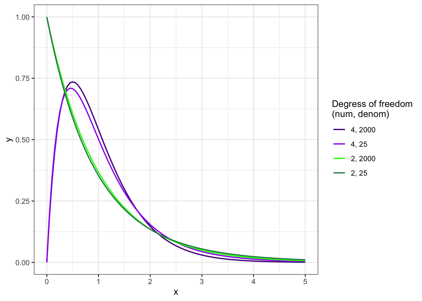
R Code 7.10 : F-distribution examples
ggplot2::ggplot(
tibble::tibble(x = c(0, 5)),
ggplot2::aes(x = x,
color = "text")
) +
ggplot2::stat_function(fun = df,
args = list(df1 = 4, df2 = 2000),
ggplot2::aes(color = "4, 2000"),
linewidth = .7) +
ggplot2::stat_function(fun = df,
args = list(df1 = 4, df2 = 25),
ggplot2::aes(color = "4, 25"),
linewidth = .7) +
ggplot2::stat_function(fun = df,
args = list(df1 = 2, df2 = 2000),
ggplot2::aes(color = "2, 2000"),
linewidth = .7) +
ggplot2::stat_function(fun = df,
args = list(df1 = 2, df2 = 25),
ggplot2::aes(color = "2, 25"),
linewidth = .7) +
ggplot2::scale_color_manual(
name = "Degress of freedom\n(num, denom)",
values = c("purple4", "purple", "green", "seagreen"),
breaks = c("4, 2000","4, 25","2, 2000", "2, 25")
)
R Code 7.11 : F-distribution for the technology use by degree ANOVA (df = 4 and 1404)
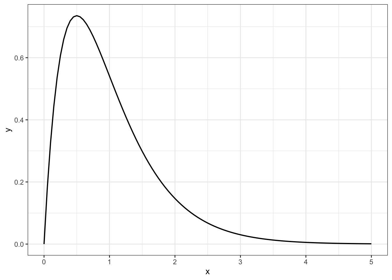
The F-distribution in Graph 7.5 suggested the F-statistic of 43.30 was far to the right in the tail of the distribution. The probability of an F-statistic this large or larger if the null were true was reported in the output as < 2.2e-16, which is < .001. With a p-value this tiny, the F-statistic would be considered statistically significant.
The mean time spent on technology use was significantly different across degree groups [F(4, 1404) = 43.3; p < .05], indicating that these groups likely came from a population with different mean time spent on technology use by educational attainment. The highest mean was the percent of time used for technology by those with graduate degrees. The lowest mean was the percent of time used for technology by those with less than a high school diploma.
ANOVA is — similar as the chi-squared test — an omnibus test: iIt identifies whether there are any differences, but doesn’t give any information about what is driving the significant results.
There are two main ways to determine where significant differences among groups are following a significant omnibus test:
There are several different types of post hoc tests, and one of the more commonly used is the Bonferroni post hoc test.
The Bonferroni adjustment multiplies each p-value from each t-test by the overall number of t-tests conducted. There were 10 pairwise comparisons (5 groups each pairwise = 5 * 2), so these p-values have been multiplied by 10. Higher p-values will not reach the threshold for statistical significance as often. Sometimes there are resulting p-values of 1.0000. As the p-value cannot be over 1, so for p-values that are over 1 when adjusted by the multiplication, they are rounded to exactly 1.0000.
R Code 7.12 : Bonferroni post hoc test
stats::pairwise.t.test(
x = gss_2018_clean$USETECH,
g = gss_2018_clean$DEGREE,
p.adjust.method = "bonferroni"
)#>
#> Pairwise comparisons using t tests with pooled SD
#>
#> data: gss_2018_clean$USETECH and gss_2018_clean$DEGREE
#>
#> < high school high school junior college bachelor
#> high school 3.8e-11 - - -
#> junior college 2.8e-15 0.0022 - -
#> bachelor < 2e-16 8.0e-13 1.0000 -
#> graduate < 2e-16 7.3e-09 1.0000 1.0000
#>
#> P value adjustment method: bonferroniThe output is different from previous statistical testing. Instead of a test statistic like t or F, the output is a matrix of p-values.
The adjusted p-values for seven of the t-tests fall below .05 and so indicate that the difference in mean time using technology between two groups is statistically significant.
For the report it would be more informative if one could add the group means for the interpretation:
#> # A tibble: 5 × 2
#> DEGREE group_means
#> <fct> <dbl>
#> 1 < high school 24.8
#> 2 high school 49.6
#> 3 junior college 62.4
#> 4 bachelor 67.9
#> 5 graduate 68.7Mean percentage of time using technology at work was statistically significantly (p < .05) lower for people with less educational attainment than a high school diploma (m = 24.8) compared to each of the other groups, where the mean percentage of time using technology ranged from 49.6 to 68.7.
Tukey’s HSD post hoc test is a modified t-test with the test statistic, q. The q test statistic formula is the same as some versions of t, but the q-distribution is different from the t-distribution, raising the critical value necessary to reach statistical significance. Even with the same test statistic, it is more difficult to reach statistical significance with a Tukey’s HSD q-statistic compared to a t-test.
\[ q = \frac{m_{1} - m_{2}}{se} \tag{7.3}\]
The stats::TukeyHSD() function does not work well with the stats::oneway.test() output from earlier, so the entire ANOVA model has to be re-estimated. The stats:aov() function works and takes similar arguments to the stats::oneway.test() function, so nesting the stats::aov() inside the stats::TukeyHSD() is one way to go.
Difference between test and fitting a model
After my first reading it wasn’t quite clear for me what the difference is between stats::oneway.test() and stats::aov().
Later — when I worked on the two-way ANOVA in Section 7.10 — I learned that the first approach is a test whereas the second functions fits a model by a call to lm(). To get the full data for testing if the data are statistically significant one has to wrap stats::aov() into to the base::summary() function.
gss_2018_clean <- base::readRDS("data/chap07/gss_2018_clean.rds")
glue::glue("################## oneway.test() ####################")
stats::oneway.test(
formula = USETECH ~ DEGREE,
data = gss_2018_clean,
var.equal = TRUE
)
glue::glue(" ")
glue::glue("###################### aov() ##########################")
glue::glue(" ")
stats::aov(
formula = USETECH ~ DEGREE,
data = gss_2018_clean
)
glue::glue(" ")
glue::glue("################## summary(aov()) ####################")
glue::glue(" ")
base::summary(
stats::aov(
formula = USETECH ~ DEGREE,
data = gss_2018_clean
)
)#> ################## oneway.test() ####################
#>
#>  One-way analysis of means
#>
#> data:  USETECH and DEGREE
#> F = 43.304, num df = 4, denom df = 1404, p-value < 2.2e-16
#>
#>
#> ###################### aov() ##########################
#>
#> Call:
#> stats::aov(formula = USETECH ~ DEGREE, data = gss_2018_clean)
#>
#> Terms:
#> DEGREE Residuals
#> Sum of Squares 221300.6 1793757.2
#> Deg. of Freedom 4 1404
#>
#> Residual standard error: 35.7436
#> Estimated effects may be unbalanced
#> 936 observations deleted due to missingness
#>
#> ################## summary(aov()) ####################
#>
#> Df Sum Sq Mean Sq F value Pr(>F)
#> DEGREE 4 221301 55325 43.3 <2e-16 ***
#> Residuals 1404 1793757 1278
#> ---
#> Signif. codes: 0 '***' 0.001 '**' 0.01 '*' 0.05 '.' 0.1 ' ' 1
#> 936 observations deleted due to missingnessR Code 7.13 : Compute Tukey’s Honestly Significance Difference (HSD)
#>   Tukey multiple comparisons of means
#>     95% family-wise confidence level
#>
#> Fit: stats::aov(formula = USETECH ~ DEGREE, data = gss_2018_clean)
#>
#> $DEGREE
#>                                    diff       lwr      upr     p adj
#> high school-< high school    24.8247754 15.145211 34.50434 0.0000000
#> junior college-< high school 37.6070313 25.201887 50.01218 0.0000000
#> bachelor-< high school       43.0859568 32.653180 53.51873 0.0000000
#> graduate-< high school       43.9107249 32.256416 55.56503 0.0000000
#> junior college-high school   12.7822558  3.362603 22.20191 0.0020352
#> bachelor-high school         18.2611813 11.651711 24.87065 0.0000000
#> graduate-high school         19.0859494 10.679691 27.49221 0.0000000
#> bachelor-junior college       5.4789255 -4.713166 15.67102 0.5833665
#> graduate-junior college       6.3036936 -5.135659 17.74305 0.5592907
#> graduate-bachelor             0.8247681 -8.438819 10.08835 0.9992282
The number of significant results of the 10 test are the same, although the Bonferroni test is more conservative. For example the p-value of the pairwise test between junior college and bachelor are 0.58 in HSD but 1.0 in Bonferroni.
The mean time spent on technology use was significantly different across education groups [F(4, 1404) = 43.3; p < .05], indicating that these groups likely came from a population with different mean time spent on technology use depending on educational attainment. The highest mean was 68.7% of time used for technology for those with graduate degrees. The lowest mean was 24.8% of the time for those with less than a high school diploma. Mean percentage of time using technology was statistically significantly (p < .05) lower for people with less than a high school diploma (m = 24.8) compared to each of the other groups where the mean percentage of time using technology ranged from 49.6 to 68.7.
Planned comparisons are computed by developing contrasts that specify which means to compare to which other means.
Bullet List
For example, to compare all the college groups to the high school group, the contrast would omit the less than high school group and compare the mean for everyone in the high school group to the mean of the combined three college groups: junior college, bachelor, and graduate.
The three categories represented by –1 will be grouped together because they are all represented by the same number.
Example 7.3 : Planned contrasts of using technology by degree
R Code 7.14 : Planned contrasts of using technology for the college groups to high school group
## 1. put the contrast into a vector
contrast1 <- c(0, 3, -1, -1, -1)

## 2. link the contrast to the categorical variable using contrasts()
stats::contrasts(x = gss_2018_clean$DEGREE) <- contrast1

## 2a. view the structure of the DEGREE variable with contrast
glue::glue("************** View the structure of DEGREE variable *****************")
utils::str(object = gss_2018_clean$DEGREE)

## 3. re-run the model using aov()
usetech_degree_aov <- stats::aov(
    formula = USETECH ~ DEGREE,
    data = gss_2018_clean
)

## 4. apply the contrasts to the aov object
glue::glue(" ")
glue::glue("******************* Summarize the aov object ****************************")
stats::summary.aov(
    object = usetech_degree_aov,
    split = list(DEGREE =
            list("high school vs. all college" = 1)))
#> ************** View the structure of DEGREE variable *****************
#> Factor w/ 5 levels "< high school",..: 3 2 4 4 5 4 2 2 1 2 ...
#> - attr(*, "contrasts")= num [1:5, 1:4] 0 3 -1 -1 -1 ...
#> ..- attr(*, "dimnames")=List of 2
#> .. ..$ : chr [1:5] "< high school" "high school" "junior college" "bachelor" ...
#> .. ..$ : NULL
#>
#> ******************* Summarize the aov object ****************************
#> Df Sum Sq Mean Sq F value Pr(>F)
#> DEGREE 4 221301 55325 43.30 < 2e-16 ***
#> DEGREE: high school vs. all college 1 64411 64411 50.41 1.97e-12 ***
#> Residuals 1404 1793757 1278
#> ---
#> Signif. codes: 0 '***' 0.001 '**' 0.01 '*' 0.05 '.' 0.1 ' ' 1
#> 936 observations deleted due to missingnessThe output showed that mean technology use for those who finished high school was statistically significantly different from mean technology use for the three college groups combined [F(1, 1404) = 50.41; p < .001].
To understand more of what was happening we need to lookat the means being compared with this contrast.
R Code 7.15 : Using technology for the recoded planned contrast between college groups to high school group
#> # A tibble: 3 × 3
#>   DEGREE        mean_usetech sd_usetech
#>   <fct>                <dbl>      <dbl>
#> 1 < high school         24.8       36.2
#> 2 high school           49.6       38.6
#> 3 all college           67.0       32.3
I have used here the first time the forcats::fct_collaps() function. This is more understandable as the option in the book, where (a) all factors are recoded and the thre highest factors with the same name “all college”.
The difference between the mean technology use time for high school (m = 49.61) compared to all college groups combined (m = 66.97) is pretty large.
R Code 7.16 : Plot of using technology for the recoded planned contrast between college groups to high school group
gss_2018_clean |>
    dplyr::mutate(DEGREE =
          forcats::fct_collapse(DEGREE,
                `all college` = c(
                    "junior college",
                    "bachelor",
                    "graduate"
                    )
                )
          ) |>
    dplyr::filter(DEGREE == "high school" | DEGREE == "all college") |>

    ggplot2::ggplot(
        ggplot2::aes(
            y = USETECH,
            x = DEGREE,
            fill = DEGREE,
            color = DEGREE
        )
    ) +
    ggplot2::geom_boxplot(
        alpha = .4,
        na.rm = TRUE
        ) +
    ggplot2::geom_jitter(
        alpha = .6,
        na.rm = TRUE
        ) +
    ggplot2::scale_fill_manual(
        values = c("gray70", "#7463AC"),
        guide = "none"
        ) +
    ggplot2::scale_color_manual(
        values = c("gray70", "#7463AC"),
        guide = "none"
        ) +
    ggplot2::labs(
        x = "Educational attainment",
        y = "Percent of time spent using technology"
        )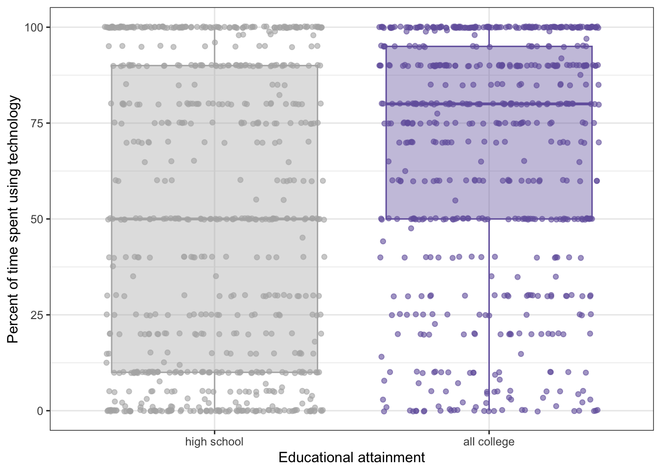
It is clear that the means of these two groups are different. The same probably would also be true for the less than high school group with the three college groups.
R Code 7.17 : Planned contrasts of time using technology on the job between college groups to less than high school group
## 1. less than high school v. all college contrast
contrast2 <- base::c(3, 0, -1, -1, -1)

## 2. bind the two contrasts together (matrix required!)
my_contrasts <-
    as.matrix(dplyr::bind_cols(
        contrast1 = contrast1,
        contrast2 = contrast2))

## 3. connect the tibble with factor variable
stats::contrasts(gss_2018_clean$DEGREE) <-  my_contrasts

## 4. compute ANOVA with planned contrasts
stats::summary.aov(
    object = usetech_degree_aov,
    split = list(DEGREE =
            list("high school vs. all college" = 1,
                 "< high school vs. all college" = 2)
            )
    )
#> Df Sum Sq Mean Sq F value Pr(>F)
#> DEGREE 4 221301 55325 43.30 < 2e-16
#> DEGREE: high school vs. all college 1 64411 64411 50.41 1.97e-12
#> DEGREE: < high school vs. all college 1 20188 20188 15.80 7.39e-05
#> Residuals 1404 1793757 1278
#>
#> DEGREE ***
#> DEGREE: high school vs. all college ***
#> DEGREE: < high school vs. all college ***
#> Residuals
#> ---
#> Signif. codes: 0 '***' 0.001 '**' 0.01 '*' 0.05 '.' 0.1 ' ' 1
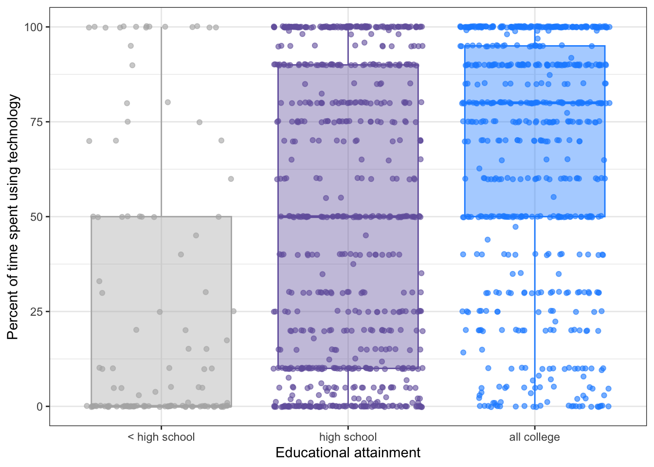
#> 936 observations deleted due to missingnessR Code 7.18 : Plot of using technology for the recoded planned contrast between college groups to less than high school group
gss_2018_clean |>
    dplyr::mutate(DEGREE =
          forcats::fct_collapse(DEGREE,
                `all college` = c(
                    "junior college",
                    "bachelor",
                    "graduate"
                    )
                )
          ) |>

    ggplot2::ggplot(
        ggplot2::aes(
            x = DEGREE,
            y = USETECH,
            fill = DEGREE,
            color = DEGREE
        )
    ) +
    ggplot2::geom_boxplot(
        alpha = .4,
        na.rm = TRUE
        ) +
    ggplot2::geom_jitter(
        alpha = .6,
        na.rm = TRUE
        ) +
    ggplot2::scale_fill_manual(
        values = c("gray70", "#7463AC", "dodgerblue"),
        guide = "none"
        ) +
    ggplot2::scale_color_manual(
        values = c("gray70", "#7463AC", "dodgerblue"),
        guide = "none"
        ) +
    ggplot2::labs(
        x = "Educational attainment",
        y = "Percent of time spent using technology"
        )
R Code 7.19 : Four planned comparisons
#>      c1 c2 c3 c4
#> [1,]  2  0  0  0
#> [2,] -1  3  0  0
#> [3,] -1 -1  2  0
#> [4,]  0 -1 -1 -1
#> [5,]  0 -1 -1  1
Procedure 7.2 : Check the values of the contrasts
ad 1: The vectors are now columns. An example of a check is to sum the column c1: \(2 + (-1) + (-1) + 0 + 0 = 0\). Columns c2, c3 and c4 also result to \(0\). So the first check conditions was passed.
ad 2: Now we have to multiply the values row-wise: \(2 \times 0 \times 0 \times 0 = 0\) It is easy to check: Whenever there is \(0\) in one of the columns then the result is also \(0\). Adding all these products together results in \(0 + 0 + 0 + 0 + 0 = 0\), so the second requirement is also met.
R Code 7.20 : Conncet the matrix with all levels of the factor variable
## connect the matrix with the factor variable
stats::contrasts(x = gss_2018_clean$DEGREE) <- conts

## estimate the ANOVA with 4 independent contrasts
usetech_degree_4_contrasts <-
    summary.aov(object = usetech_degree_aov,
        split = list(DEGREE =
             list("< high school vs. high school & jr college" = 1,
                  "high school vs. all college" = 2,
                  "jr college vs. bach or grad degree" = 3,
                  "bachelor’s vs. graduate degree" = 4)
             )
        )
usetech_degree_4_contrasts
#> Df Sum Sq Mean Sq
#> DEGREE 4 221301 55325
#> DEGREE: < high school vs. high school & jr college 1 64411 64411
#> DEGREE: high school vs. all college 1 20188 20188
#> DEGREE: jr college vs. bach or grad degree 1 63902 63902
#> DEGREE: bachelor’s vs. graduate degree 1 72800 72800
#> Residuals 1404 1793757 1278
#> F value Pr(>F)
#> DEGREE 43.30 < 2e-16 ***
#> DEGREE: < high school vs. high school & jr college 50.41 1.97e-12 ***
#> DEGREE: high school vs. all college 15.80 7.39e-05 ***
#> DEGREE: jr college vs. bach or grad degree 50.02 2.40e-12 ***
#> DEGREE: bachelor’s vs. graduate degree 56.98 7.88e-14 ***
#> Residuals
#> ---
#> Signif. codes: 0 '***' 0.001 '**' 0.01 '*' 0.05 '.' 0.1 ' ' 1
#> 936 observations deleted due to missingnessR Code 7.21 : Adjust p-values for multiple comparisons
adj_p_values <- stats::p.adjust(
    p = usetech_degree_4_contrasts[[1]][["Pr(>F)"]],
    method = "bonferroni"
    )
adj_p_values
#>
#> 1.329994e-33
#> < high school vs. high school & jr college
#> 9.850341e-12
#> high school vs. all college
#> 3.696043e-04
#> jr college vs. bach or grad degree
#> 1.198280e-11
#> bachelor’s vs. graduate degree
#> 3.939123e-13
#>
#> NAThe adjusted p-values were still very small, so the conclusions about statistical significance did not change, even when using a conservative adjustment like Bonferroni.
R Code 7.22 : Visualizing the distribution of technology use at work by educational attainment for four planned comparisons
## < high school / hs & jr college ########
gg_violin1 <- gss_2018_clean |>
  dplyr::mutate(DEGREE =
        dplyr::if_else(DEGREE == "< high school", "< high school",
        dplyr::if_else(DEGREE %in% c("high school",
                                     "junior college"),
                                     "high school & jr college",
                                     NA))) |>
  dplyr::mutate(DEGREE =
         base::factor(DEGREE, levels = c("< high school",
                                         "high school & jr college"),
                                         ordered = T)) |>
  dplyr::filter(DEGREE == "< high school" |
                DEGREE == "high school & jr college") |>

      ggplot2::ggplot(
        ggplot2::aes(
            y = USETECH,
            x = DEGREE,
            fill = DEGREE,
            color = DEGREE
        )
    ) +
    ggplot2::geom_violin(
        alpha = .4,
        na.rm = TRUE
        ) +
    ggplot2::geom_jitter(
        alpha = .6,
        na.rm = TRUE
        ) +
    ggplot2::scale_fill_manual(
        values = c("gray70", "#7463AC"),
        guide = "none"
        ) +
    ggplot2::scale_color_manual(
        values = c("gray70", "#7463AC"),
        guide = "none"
        ) +
    ggplot2::labs(
        x = "Educational attainment",
        y = "Percent of time spent using technology"
        )


## high school & three college groups##########
gg_violin2 <- gss_2018_clean |>
    dplyr::mutate(DEGREE =
          forcats::fct_collapse(DEGREE,
                `all college` = c(
                    "junior college",
                    "bachelor",
                    "graduate"
                    )
                )
          ) |>
    dplyr::filter(DEGREE == "high school" | DEGREE == "all college") |>
    ggplot2::ggplot(
        ggplot2::aes(
            y = USETECH,
            x = DEGREE,
            fill = DEGREE,
            color = DEGREE
        )
    ) +
    ggplot2::geom_violin(
        alpha = .4,
        na.rm = TRUE
        ) +
    ggplot2::geom_jitter(
        alpha = .6,
        na.rm = TRUE
        ) +
    ggplot2::scale_fill_manual(
        values = c("gray70", "#7463AC"),
        guide = "none"
        ) +
    ggplot2::scale_color_manual(
        values = c("gray70", "#7463AC"),
        guide = "none"
        ) +
    ggplot2::labs(
        x = "Educational attainment",
        y = "Percent of time spent using technology"
        )

## jr college & bachelor & graduate ##########
gg_violin3 <- gss_2018_clean |>
    dplyr::mutate(DEGREE =
    dplyr::if_else(DEGREE %in% c("< high school", "high school"), NA,
    dplyr::if_else(DEGREE == "junior college", "jr college",
    dplyr::if_else(DEGREE %in% c("bachelor", "graduate"),
                                 "bachelor or graduate", NA)))) |>
    dplyr::mutate(DEGREE =
      base::factor(DEGREE,
                   levels = c("jr college",
                              "bachelor or graduate",
                              ordered = T))) |>
    dplyr::filter(DEGREE == "jr college" | DEGREE == "bachelor or graduate") |>

    ggplot2::ggplot(
        ggplot2::aes(
            y = USETECH,
            x = DEGREE,
            fill = DEGREE,
            color = DEGREE
        )
    ) +
    ggplot2::geom_violin(
        alpha = .4,
        na.rm = TRUE
        ) +
    ggplot2::geom_jitter(
        alpha = .6,
        na.rm = TRUE
        ) +
    ggplot2::scale_fill_manual(
        values = c("gray70", "#7463AC"),
        guide = "none"
        ) +
    ggplot2::scale_color_manual(
        values = c("gray70", "#7463AC"),
        guide = "none"
        ) +
    ggplot2::labs(
        x = "Educational attainment",
        y = "Percent of time spent using technology"
        )

## bachelor & graduate ############
gg_violin4 <- gss_2018_clean |>
    dplyr::mutate(DEGREE =
        dplyr::if_else(DEGREE == "bachelor", "bachelor",
        dplyr::if_else(DEGREE == "graduate", "graduate", NA))) |>
      dplyr::mutate(DEGREE =
        base::factor(DEGREE,
                     levels = c("bachelor",
                                "graduate",
                                ordered = T))) |>
    dplyr::filter(DEGREE == "bachelor" | DEGREE == "graduate") |>

    ggplot2::ggplot(
        ggplot2::aes(
            y = USETECH,
            x = DEGREE,
            fill = DEGREE,
            color = DEGREE
        )
    ) +
    ggplot2::geom_violin(
        alpha = .4,
        na.rm = TRUE
        ) +
    ggplot2::geom_jitter(
        alpha = .6,
        na.rm = TRUE
        ) +
    ggplot2::scale_fill_manual(
        values = c("gray70", "#7463AC"),
        guide = "none"
        ) +
    ggplot2::scale_color_manual(
        values = c("gray70", "#7463AC"),
        guide = "none"
        ) +
    ggplot2::labs(
        x = "Educational attainment",
        y = "Percent of time spent using technology"
        )

gridExtra::grid.arrange(
    gg_violin1, gg_violin2,
    gg_violin3, gg_violin4,
    ncol = 2)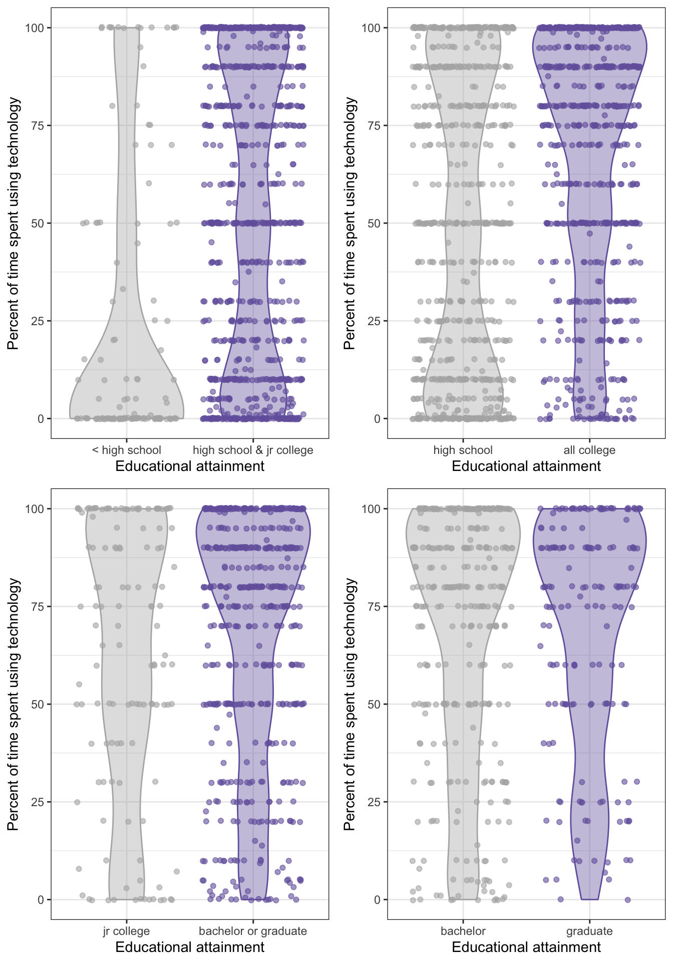
This is the replication of book’s Figure 7.10.
R Code 7.23 : Summary of the constrasts statistic
## contrast 1 statistics ###########
glue::glue(" ")
glue::glue("#################### contrast 1 statistics ###################")
gss_2018_clean  |>
  dplyr::mutate(DEGREE =
        dplyr::if_else(DEGREE == "< high school", "< high school",
        dplyr::if_else(DEGREE %in% c("high school",
                                     "junior college"),
                                     "high school & jr college",
                                     NA))) |>
  dplyr::mutate(DEGREE =
         base::factor(DEGREE, levels = c("< high school",
                                         "high school & jr college"),
                                         ordered = T)) |>
  dplyr::group_by(DEGREE) |>
  dplyr::summarise(
      mean_usetech = base::mean(x = USETECH, na.rm = T),
      sd_usetech = stats::sd(x = USETECH, na.rm = T))


## contrast 2 statistics ##############
glue::glue(" ")
glue::glue("#################### contrast 2 statistics ###################")
gss_2018_clean |>
  dplyr::mutate(DEGREE =
         base::factor(DEGREE, labels = c(NA,
               "high school", "all college",
               "all college", "all college"),
               ordered = T)) |>
  dplyr::group_by(DEGREE) |>
  dplyr::summarise(
      mean_usetech = mean(x = USETECH, na.rm = T),
      sd.usetech = sd(x = USETECH, na.rm = T))

## contrast 3 statistics ##############
glue::glue(" ")
glue::glue("#################### contrast 3 statistics ###################")
gss_2018_clean |>
  dplyr::mutate(DEGREE =
    dplyr::if_else(DEGREE %in% c("< high school", "high school"), NA,
    dplyr::if_else(DEGREE == "junior college", "jr college",
    dplyr::if_else(DEGREE %in% c("bachelor", "graduate"),
                                 "bach or grad degree", NA)))) |>
    dplyr::mutate(DEGREE =
      base::factor(DEGREE,
                   levels = c("jr college",
                              "bach or grad degree",
                              ordered = T))) |>
  dplyr::group_by(DEGREE) |>
  dplyr::summarise(
      mean_usetech = mean(x = USETECH, na.rm = T),
      sd.usetech = sd(x = USETECH, na.rm = T))

# contrast 4 statistics ####################
glue::glue(" ")
glue::glue("#################### contrast 4 statistics ###################")
gss_2018_clean |>
  dplyr::mutate(DEGREE =
    dplyr::if_else(DEGREE == "bachelor", "bachelor",
    dplyr::if_else(DEGREE == "graduate", "graduate", NA))) |>
  dplyr::mutate(DEGREE =
    base::factor(DEGREE,
                 levels = c("bachelor",
                            "graduate",
                            ordered = T))) |>
  dplyr::group_by(DEGREE) |>
  dplyr::summarise(
     mean_usetech = mean(x = USETECH, na.rm = T),
     sd_usetech = sd(x = USETECH, na.rm = T))
#>
#> #################### contrast 1 statistics ###################
#> # A tibble: 3 × 3
#> DEGREE mean_usetech sd_usetech
#> <ord> <dbl> <dbl>
#> 1 < high school 24.8 36.2
#> 2 high school & jr college 51.7 38.4
#> 3 <NA> 68.2 31.4
#>
#> #################### contrast 2 statistics ###################
#> # A tibble: 3 × 3
#> DEGREE mean_usetech sd.usetech
#> <ord> <dbl> <dbl>
#> 1 <NA> 24.8 36.2
#> 2 high school 49.6 38.6
#> 3 all college 67.0 32.3
#>
#> #################### contrast 3 statistics ###################
#> # A tibble: 3 × 3
#> DEGREE mean_usetech sd.usetech
#> <fct> <dbl> <dbl>
#> 1 jr college 62.4 35.2
#> 2 bach or grad degree 68.2 31.4
#> 3 <NA> 45.8 39.3
#>
#> #################### contrast 4 statistics ###################
#> # A tibble: 3 × 3
#> DEGREE mean_usetech sd_usetech
#> <fct> <dbl> <dbl>
#> 1 bachelor 67.9 32.1
#> 2 graduate 68.7 30.2
#> 3 <NA> 48.1 39.1The mean time spent on technology use at work was significantly different across educational attainment groups [F(4, 1404) = 43.3; p < .05], indicating these groups likely came from populations with different mean time spent on technology use. The highest mean was percent of time used for technology for those with graduate degrees. The lowest mean was percent of time for those with less than a high school diploma. A set of planned comparisons found that the mean time spent using technology was statistically significantly (p < .05) lower for (a) those with < high school education (m = 24.8) compared to those with high school or junior college (m = 51.7), (b) those with a high school education (m = 49.61) compared to those with all college groups combined (m = 67.0), (c) those with a junior college degree (m = 62.4) compared to those with a bachelor’s or graduate degree (m = 68.2), and (d) those with a bachelor’s degree (m = 67.9) compared to those with a graduate degree (m = 68.7). Overall, the patterns show statistically significant increases in time spent using technology at work for those with more education.
How many contrasts could be done and how all these statistical comparisons might be inflating the Type I error? — In addition to each comparison comparing two things and each comparison adding to zero, the planned comparisons as a group should isolate each group (e.g., the high school group) only one time. This ensures that the contrasts are independent of each other since the variance for each group is only used by itself in a statistical comparison one time. Because each group is isolated one time, the total maximum number of contrasts allowable is one less than the number of groups.
When you have hypotheses ahead of time about which groups are different from one another, use planned comparisons. When you do not have hypotheses ahead of time about which means are different from each other, use post hoc tests if the ANOVA has a statistically significant F-statistic. Good research practices suggest that having hypotheses ahead of time is a stronger strategy unless the research is truly exploratory.
Bullet List
Similar as the effect size Cramér’s V for chi-squared tests and Cohen’s d for t-test, there are also effect size indices for ANOVA:
Formula 7.3 : Formula for omega-squared
\[ \omega^2 = \frac{F - 1}{f + \frac{n-k+1}{k-1}} \tag{7.4}\]
R Code 7.24 : Manual computation of effect size omega-squared
gss_2018_clean <- base::readRDS("data/chap07/gss_2018_clean.rds")

usetech_degree_aov <- stats::aov(
    formula = USETECH ~ DEGREE,
    data = gss_2018_clean
)

glue::glue("############# ANOVA model USETECH ~ DEGREE ##################")
(
    usetech_degree_aov_summary <- base::summary(usetech_degree_aov)
)

F_value = usetech_degree_aov_summary[[1]][["F value"]][[1]]
n = base::nrow(usetech_degree_aov[["model"]])
k = usetech_degree_aov[["rank"]]


glue::glue(" ")
glue::glue("############# Omega-squared ##################")
omega_squared <- (F_value - 1) / (F_value + ((n - k + 1) / (k - 1)))
omega_squared
#> ############# ANOVA model USETECH ~ DEGREE ##################
#> Df Sum Sq Mean Sq F value Pr(>F)
#> DEGREE 4 221301 55325 43.3 <2e-16 ***
#> Residuals 1404 1793757 1278
#> ---
#> Signif. codes: 0 '***' 0.001 '**' 0.01 '*' 0.05 '.' 0.1 ' ' 1
#> 936 observations deleted due to missingness
#>
#> ############# Omega-squared ##################
#> [1] 0.1072194WATCH OUT! Error in the book’s calculation
In the first term in the book -1 is missing! The formula is F-1 that should be therefore (summ.tech.anova[[1]][1, 4] -1).
With this correction we get the same value as in the manual calculation: 0.1072194.
Assessment 7.1 : Interpretation of omega-squared effect size
This is quite similar to the eta_squared (\(\eta^2\)) assessment as listed in Computation of Effect Sizes.
The mean time spent on technology use at work was significantly different across educational attainment groups [F(4, 1404) = 43.3; p < .05], indicating these groups likely came from populations with different mean time spent on technology use. The highest mean was percent of time used for technology for those with graduate degrees. The lowest mean was percent of time for those with less than a high school diploma. A set of planned comparisons found that the mean time spent using technology was statistically significantly (p < .05) lower for (a) those with < high school education (m = 24.8) compared to those with high school or junior college (m = 51.7), (b) those with a high school education (m = 49.61) compared to those with all college groups combined (m = 67.0), (c) those with a junior college degree (m = 62.4) compared to those with a bachelor’s or graduate degree (m = 68.2), and (d) those with a bachelor’s degree (m = 67.9) compared to those with a graduate degree (m = 68.7). Overall, the patterns show statistically significant increases in time spent using technology at work for those with more education. The strength of the relationship between degree and time using technology at work was medium (\(ω^2\) = .11).
Example 7.4 : Testing normality
R Code 7.25 : Testing normality with density plots
gss_2018_clean |>
    tidyr::drop_na(USETECH) |>
    ggplot2::ggplot(
        ggplot2::aes(x = USETECH)
    ) +
    ggplot2::geom_density(
        ggplot2::aes(
            fill = DEGREE
        )
    ) +
    ggplot2::facet_wrap(
        facets = ggplot2::vars(DEGREE),
        nrow = 2
    ) +
    ggokabeito::scale_fill_okabe_ito(guide = "none") +
    ggplot2::labs(
        x = "Percent of time using tech",
        y = "Probability density")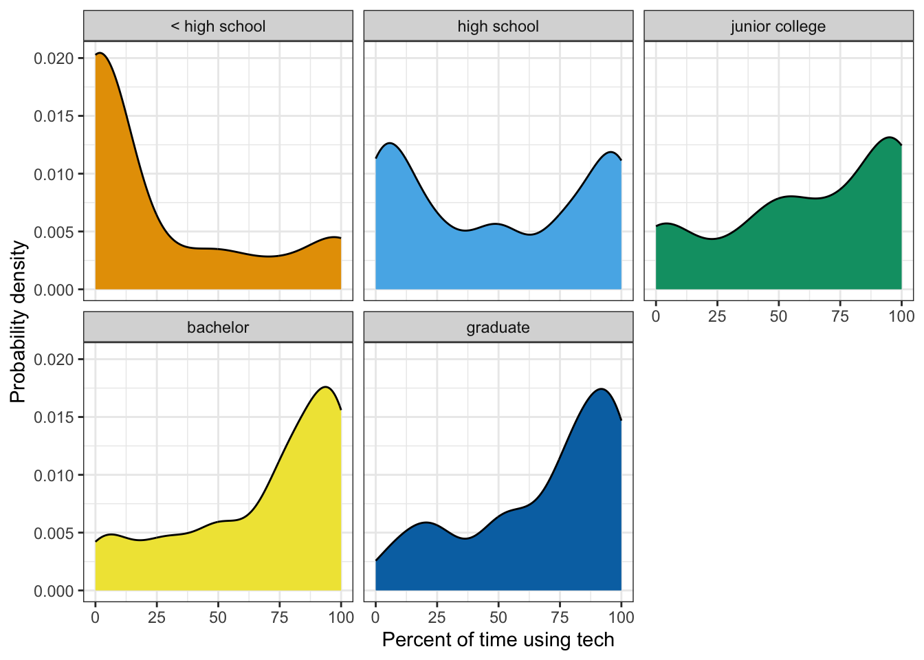
None of these graphs looks normally distributed!
R Code 7.26 : Testing normality with Q-Q plots
gss_2018_clean  |>
  tidyr::drop_na(USETECH) |>

  ggplot2::ggplot(
      ggplot2::aes(sample = USETECH)
      ) +
  ggplot2::geom_abline(
      ggplot2::aes(
          intercept = mean(USETECH),
          slope = sd(USETECH),
          linetype = "Normally distributed"),
          color = "gray60",
          linewidth = 1
      ) +
  ggplot2::stat_qq(
      ggplot2::aes(color = DEGREE)
      ) +
  ggokabeito::scale_color_okabe_ito(guide = "none") +
  ggplot2::scale_linetype_manual(
      name = "",
      values = 1) +
  ggplot2::labs(
      x = "Theoretical normal distribution",
      y = "Observed values of percent time using tech"
      ) +
  ggplot2::facet_wrap(
      facets = ggplot2::vars(DEGREE),
      nrow = 2
      )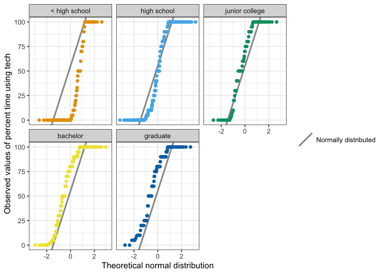
The text in the books says that “none of the groups appeared to be normally distributed based on either type of plot.” This is ok for me with the density plot. But for me with not so much experience it is difficult to decide with the small Q-Q plots.
The next tab display the Q-Q plots for each group much bigger.
R Code 7.27 : Testing normality with Q-Q plots
gss_2018_clean  |>
  tidyr::drop_na(USETECH) |>

  ggplot2::ggplot(
      ggplot2::aes(sample = USETECH)
      ) +
  ggplot2::geom_abline(
      ggplot2::aes(
          intercept = mean(USETECH),
          slope = sd(USETECH),
          linetype = "Normally distributed"),
          color = "gray60",
          linewidth = 1
      ) +
  ggplot2::stat_qq(
      ggplot2::aes(color = DEGREE)
      ) +
  ggokabeito::scale_color_okabe_ito(guide = "none") +
  ggplot2::scale_linetype_manual(
      name = "",
      values = 1) +
  ggplot2::theme(legend.position = "top") +
  ggplot2::labs(
      x = "Theoretical normal distribution",
      y = "Observed values of percent time using tech"
      ) +
  ggplot2::facet_wrap(
      facets = ggplot2::vars(DEGREE),
      nrow = 5
      )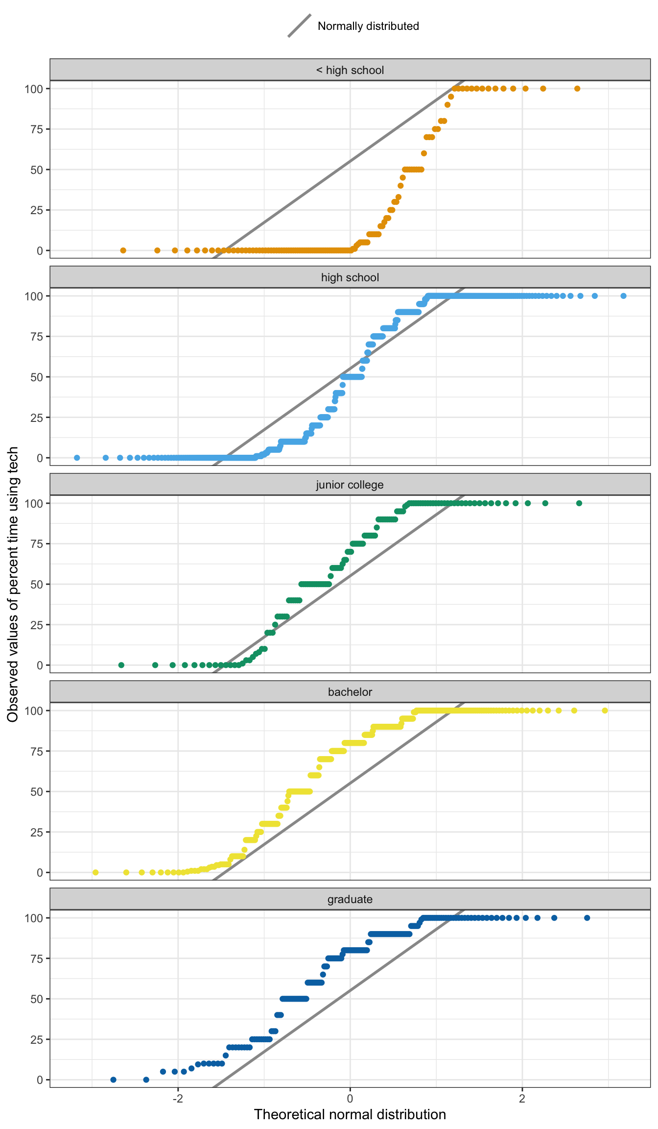
Now I can see it very clearly: All groups are not normally distributed. One can also observe that the floor and ceiling values are driving some of the non-normality.
R Code 7.28 : Numbered R Code Title
glue::glue("###### Test for the whole numeric USETECH vector #######")
stats::shapiro.test(gss_2018_clean$USETECH)

glue::glue(" ")
glue::glue("###### Test for DEGREE groups of USETECH vector #######")
gss_2018_clean |>
    dplyr::select(USETECH, DEGREE) |>
    tidyr::drop_na() |>
    dplyr::group_by(DEGREE) |>
    dplyr::summarize(
        shapiro_p_value = stats::shapiro.test(USETECH)$p.value
    )
#> ###### Test for the whole numeric USETECH vector #######
#>
#> Shapiro-Wilk normality test
#>
#> data: gss_2018_clean$USETECH
#> W = 0.8645, p-value < 2.2e-16
#>
#>
#> ###### Test for DEGREE groups of USETECH vector #######
#> # A tibble: 5 × 2
#> DEGREE shapiro_p_value
#> <fct> <dbl>
#> 1 < high school 1.83e-14
#> 2 high school 5.99e-24
#> 3 junior college 2.92e- 9
#> 4 bachelor 1.22e-16
#> 5 graduate 4.34e-11In contrast with the systolic blood pressure data we have this time less than 5,000 observations and can therefore apply the Shapiro-Wilk test (see Section 6.9.3.2).
All five of the Shapiro-Wilk tests were statistically significant, indicating that the null hypothesis for this test (i.e., the data are normally distributed) has to be rejected for each group.
The data need to be not only normally distributed, but also spread out equally in each group, e.g. we need equal variances across groups.
R Code 7.29 : Levene’s test: Testing homogeneity of variances
car::leveneTest(
    y = USETECH ~ DEGREE,
    data = gss_2018_clean,
    center = mean)
#> Levene's Test for Homogeneity of Variance (center = mean)
#> Df F value Pr(>F)
#> group 4 18.312 1.121e-14 ***
#> 1404
#> ---
#> Signif. codes: 0 '***' 0.001 '**' 0.01 '*' 0.05 '.' 0.1 ' ' 1The p-value for the Levene’s test suggests that we need to reject the null hypothesis. The variances of the USETECH variable are statistically significantly different across groups (p < .05). The ANOVA fails the assumption of homogeneity of variances.
There are several tests available when the assumption of homogeneity fails. The book mentions two but there are others as well:
stats::oneway.test() and onewaytests::bf.test()
stats::oneway.test() with var.equal = FALSE, and onwaytests::welch.test(),car::leveneTest() with center = median (default), onewaytests::homog.test() with method = "Levene".onewaytests::homog.test() with method = "Bartlett"
onewaytests::homog.test() with method = "Fligner"
The Brown-Forsythe F-statistic uses the distance each observation has from the median of the variable. The alternate F-statistic is then computed using the same F formula but with the means computed from the distance to the median instead using the raw values of the continuous variable.
Resource 7.2 Packages for Brown-Forsythe F-statistic
There are several packages with Brown-Forsythe F-statistic. Most of the explanations and examples in the internet propose {onewaytests}. Although this package has a low download figure under 100, I have added it to my package description in Appendix A, because it includes many tests specialized for ANOVA with failed assumptions.
Instead of the Brown-Forsythe F-statistic one could also use Levene’s test from the {car} packages with the argument center = median.
Both Levene’s test and Brown-Forsythe test can be used for testing for homogeneity of variances on nonnormal data. But, the Brown-Forsythe test is more robust than Levene’s test when data distributions are skewed or heavy-tailed (Cauchy distribution). Brown-Forsythe test is a modified version of Levene’s test. (Brown-Forsythe test for equality of variances in R) (Bedre 2016).
The {CGPfunctions} can’t be downloaded from CRAN beginning with R version 4.0, but you could use the GitHub version after you installed the {pwr} package. (See issue #44).
#> # A tibble: 6 × 4
#>   package      average from       to
#>   <chr>          <dbl> <date>     <date>
#> 1 car            13044 2024-03-21 2024-03-27
#> 2 onewaytests       82 2024-03-21 2024-03-27
#> 3 ALSM              49 2024-03-21 2024-03-27
#> 4 CGPfunctions      39 2024-03-21 2024-03-27
#> 5 doex              14 2024-03-21 2024-03-27
#> 6 homnormal 6 2024-03-21 2024-03-27Welchs’s F-statistic is an alternate F-statistic used in analysis of variance when the assumption of homogeneity of variance is not met. The calculations for the Welch’s F-statistic use weights to calculate the group means and the grand mean.
Instead of using the complex formula it is better to use R functions.
Example 7.5 : Testing homogeneity of variances with different tests
NHST Step 1
Write the null and alternate hypotheses:
NHST Step 2
Compute the test statistic.
R Code 7.30 : Transform the outcome variable and use the oneway.test()
gss_2018_clean <- base::readRDS("data/chap07/gss_2018_clean.rds")

gss_2018_clean2 <- gss_2018_clean |>
    dplyr::group_by(DEGREE) |>
    dplyr::mutate(
        usetech_tran = base::abs(USETECH - median(USETECH, na.rm = TRUE))
        ) |>
    dplyr::ungroup()

save_data_file("chap07", gss_2018_clean2, "gss_2018_clean2.rds")

base::summary(gss_2018_clean2$usetech_tran)

bf_test_manual <- stats::oneway.test(
    formula = usetech_tran ~ DEGREE,
    data = gss_2018_clean2)
bf_test_manual
#> Min. 1st Qu. Median Mean 3rd Qu. Max. NA's
#> 0.00 10.00 30.00 30.22 50.00 100.00 936
#>
#> One-way analysis of means (not assuming equal variances)
#>
#> data: usetech_tran and DEGREE
#> F = 19.747, num df = 4.00, denom df = 364.77, p-value = 9.965e-15NHST Step 3
Review and interpret the test statistics: Calculate the probability that your test statistic is at least as big as it is if there is no relationship (i.e., the null is true).
The p-value in this case is much less than .05. The value of an \(F_{BF}\)-statistic being this large or larger happens a tiny percentage of the time when the null hypothesis is true.
NHST Step 4
Conclude and write report.
The results show a statistically significant difference of the means of the transformed technology use variable by educational attainment group [\(F_{BF}(4, 364.77) = 19.747; p < .05\)].
R Code 7.31 : Testing homogeneity of variances with Brown-Forsythe test from {onewaytests}
onewaytests::bf.test(
    formula = USETECH ~ DEGREE,
    data = gss_2018_clean
)
#>
#> Brown-Forsythe Test (alpha = 0.05)
#> -------------------------------------------------------------
#> data : USETECH and DEGREE
#>
#> statistic : 47.04051
#> num df : 4
#> denom df : 769.209
#> p.value : 2.152414e-35
#>
#> Result : Difference is statistically significant.
#> -------------------------------------------------------------NHST Step 1
Write the null and alternate hypotheses:
Compute the test statistic.
R Code 7.32 : Testing homogeneity of variances with Welch’s test (book version)
stats::oneway.test(
    formula = USETECH ~ DEGREE,
    data = gss_2018_clean,
    var.equal = FALSE
    )
#>
#> One-way analysis of means (not assuming equal variances)
#>
#> data: USETECH and DEGREE
#> F = 46.06, num df = 4.00, denom df = 400.31, p-value < 2.2e-16Review and interpret the test statistics: Calculate the probability that your test statistic is at least as big as it is if there is no relationship (i.e., the null is true).
The p-value in this case is < 2.2e-16, which is much less than .05. The value of an \(F_{W}\)-statistic being this large or larger happens a tiny amount of the time when the null hypothesis is true.
Conclude and write report.
The results show a statistically significant difference in the mean of the USETECH variable by degree group [\(F_{W}(4, 400.31) = 46.06; p < .05\)].
In contrast to the original ANOVA with 1404 degrees of freedom in the denominator(see: Table 7.1), we have now with 400.31 fewer degrees of freedom. With fewer degrees of freedom, the F-statistic has to be a larger number to reach statistical significance.
R Code 7.33 : Comparison of different F-distributions with 2000, 25 and 10 degrees of freedom
ggplot2::ggplot() +
  ggplot2::xlim(0, 5) +
  ggplot2::geom_function(fun = df,
                           args = list(df1 = 4, df2 = 2000),
                           ggplot2::aes(color = "4, 2000"),
                           linewidth = .7) +
    ggplot2::geom_function(fun = df,
                           args = list(df1 = 4, df2 = 25),
                           ggplot2::aes(color = "4, 25"),
                           linewidth = .7) +
    ggplot2::geom_function(fun = df,
                           args = list(df1 = 4, df2 = 10),
                           ggplot2::aes(color = "4, 10"),
                           linewidth = .7) +
    ggplot2::geom_function(fun = df,
                           args = list(df1 = 2, df2 = 2000),
                           ggplot2::aes(color = "2, 2000"),
                           linewidth = .7) +
    ggokabeito::scale_color_okabe_ito(
        name = "Degress of freedom\n(num, denominator)",
        breaks = c("4, 2000","4, 25","4, 10", "2, 2000")
    )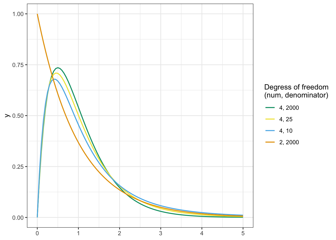
Although there isn’t much difference between three of the distributions, the area under the curves is what matters for the p-value cutoff. When the line is just slightly closer to the x-axis, this changes things quickly for the area under the curve.
The thresholds for statistical significance (p < .05) for these three lines are
The numerator degrees of freedom had a much bigger impact on the significance threshold. For example, an ANOVA with 2 degrees of freedom and the same 2000 degrees of freedom in the denominator would have a threshold for (p < .05) significance of 3.00 instead of 2.38 for the 4 and 2000 threshold. You can see the very different function curve in the graph.
R Code 7.34 : Testing homogeneity of variances with Welch’s test with {onewaytests}
onewaytests::welch.test(
    formula = USETECH ~ DEGREE,
    data = gss_2018_clean
)
#>
#> Welch's Heteroscedastic F Test (alpha = 0.05)
#> -------------------------------------------------------------
#> data : USETECH and DEGREE
#>
#> statistic : 46.06012
#> num df : 4
#> denom df : 400.3121
#> p.value : 7.87281e-32
#>
#> Result : Difference is statistically significant.
#> -------------------------------------------------------------With the exception of a smaller p-value the results are the same as with stats::oneway.test().
R Code 7.35 : Testing homogeneity of variances with different tests from the {onewaytests} package
onewaytests::homog.test(
    formula = USETECH ~ DEGREE,
    data = gss_2018_clean,
    method = "Levene"
)
#>
#> Levene's Homogeneity Test (alpha = 0.05)
#> -----------------------------------------------
#> data : USETECH and DEGREE
#>
#> statistic : 18.31161
#> num df : 4
#> denum df : 1404
#> p.value : 1.121265e-14
#>
#> Result : Variances are not homogeneous.
#> -----------------------------------------------onewaytests::homog.test(
formula = USETECH ~ DEGREE,
data = gss_2018_clean,
method = "Bartlett"
)#>
#> Bartlett's Homogeneity Test (alpha = 0.05)
#> -----------------------------------------------
#> data : USETECH and DEGREE
#>
#> statistic : 24.20202
#> parameter : 4
#> p.value : 7.27617e-05
#>
#> Result : Variances are not homogeneous.
#> -----------------------------------------------onewaytests::homog.test(
formula = USETECH ~ DEGREE,
data = gss_2018_clean,
method = "Fligner"
)#>
#> Fligner-Killeen Homogeneity Test (alpha = 0.05)
#> ---------------------------------------------------
#> data : USETECH and DEGREE
#>
#> statistic : 36.33757
#> parameter : 4
#> p.value : 2.465992e-07
#>
#> Result : Variances are not homogeneous.
#> ---------------------------------------------------The Kruskal-Wallis test is used to compare three or more groups when the normal distribution assumption fails for ANOVA. Like several of the tests used when the outcome is not normally distributed for a t-test, the Kruskal-Wallis (K-W) test compares ranks among groups. Specifically, the observations are put in order by size, and each is assigned a rank. The mean rank for each group is then computed and used to calculate the K-W test statistic, H.
Formula 7.4 : Kruskal-Wallis test
\[ H = \frac{12}{n(n+1)}\sum_{j=1}^{k}n_{j}(\bar{r_{j}}-\frac{n+1}{2})^2 \tag{7.5}\]
Write the null and alternate hypotheses:
Compute the test statistic.
Example 7.6 : Testing normality with the Kruskal-Wallis test
R Code 7.36 : Compare using technology by highest educational attainment with stats::kruskal.test()
kw_test <- stats::kruskal.test(
    formula = USETECH ~ DEGREE,
    data = gss_2018_clean
)
kw_test
#>
#> Kruskal-Wallis rank sum test
#>
#> data: USETECH by DEGREE
#> Kruskal-Wallis chi-squared = 142.21, df = 4, p-value < 2.2e-16The distribution of the H statistic is approximately a chi-squared distribution, so the R output lists “chi-squared” instead of H.
R Code 7.37 : Compare using technology by highest educational attainment with onewaytests::kw.test()
onewaytests::kw.test(
    formula = USETECH ~ DEGREE,
    data = gss_2018_clean
)
#>
#> Kruskal-Wallis Test (alpha = 0.05)
#> -------------------------------------------------------------
#> data : USETECH and DEGREE
#>
#> statistic : 142.2141
#> parameter : 4
#> p.value : 9.474913e-30
#>
#> Result : Difference is statistically significant.
#> -------------------------------------------------------------The value of the statistic is the same as with stats::kruskal.test() but the p-value is lower, e.g. it is more stringent.
Review and interpret the test statistics: Calculate the probability that your test statistic is at least as big as it is if there is no relationship (i.e., the null is true).
The p-value in both tests, as usual, is very tiny. The value of an H-statistic being this large or larger happens a tiny percentage of the time when the null hypothesis is true.
Conclude and write report.
There is a difference in the mean rank for technology use by degree group \([H(4) = 142.21; p < .05]\).
Like the ANOVA results, the Kruskal-Wallis test identifies whether there is a difference somewhere among the means, but it does not identify which groups are different from one another. A post hoc test like Bonferroni or Tukey’s HSD could help. For K-W, the Dunn’s post hoc test of multiple comparisons is useful for identifying which groups are statistically significantly different from which other groups.
Example 7.7 : Dunn’s post hoc test for Kruskal-Wallis
R Code 7.38 : Dunn’s post hoc test for Kruskal-Wallis
dunn.test::dunn.test(
    x = gss_2018_clean$USETECH,
    g = gss_2018_clean$DEGREE,
    method = "bonferroni"
)
#> Kruskal-Wallis rank sum test
#>
#> data: x and group
#> Kruskal-Wallis chi-squared = 142.2141, df = 4, p-value = 0
#>
#>
#> Comparison of x by group
#> (Bonferroni)
#> Col Mean-|
#> Row Mean | < high s bachelor graduate high sch
#> ---------+--------------------------------------------
#> bachelor | -10.43723
#> | 0.0000*
#> |
#> graduate | -9.495755 -0.191842
#> | 0.0000* 1.0000
#> |
#> high sch | -6.834568 6.465520 5.294962
#> | 0.0000* 0.0000* 0.0000*
#> |
#> junior c | -7.755300 1.244464 1.264131 -3.190136
#> | 0.0000* 1.0000 1.0000 0.0071*
#>
#> alpha = 0.05
#> Reject Ho if p <= alpha/2The Dunn’s test is a rank-sum test just like the Mann-Whitney U and can be interpreted in the same way.
No difference in technology use
Differences in technology use
There are differences in technology use between all lower educational attainments (less than high school and high school) versus the higher educational attainments (junior college, bachelor, and graduate). There are also differences between less than high school versus high high school.
There are no differences between the higher educational attainments junior college, bachelor, and graduate.
R Code 7.39 : Preparing a graphic for visualizing the differences in the Dunn test
#>    Min. 1st Qu.  Median    Mean 3rd Qu.    Max.    NA's
#>    88.5   357.5   699.5   705.0  1019.0  1272.0     936
R Code 7.40 : Visualizing the differences in the Dunn test
gss_2018_clean3 <-  base::readRDS("data/chap07/gss_2018_clean3.rds")

gss_2018_clean3 |>
  ggplot2::ggplot(
      ggplot2::aes(
          y = usetech_rank,
          x = DEGREE)
      ) +
  ggplot2::geom_jitter(
      ggplot2::aes(color = DEGREE),
      alpha = .6,
      na.rm = TRUE
      ) +
  ggplot2::geom_boxplot(
      ggplot2::aes(fill = DEGREE),
      alpha = .4,
      na.rm = TRUE
      ) +
  ggokabeito::scale_color_okabe_ito(guide = "none") +
  ggokabeito::scale_fill_okabe_ito(guide = "none") +
  ggplot2::labs(
      x = "Educational attainment",
      y = "Ranks of technology use time"
      )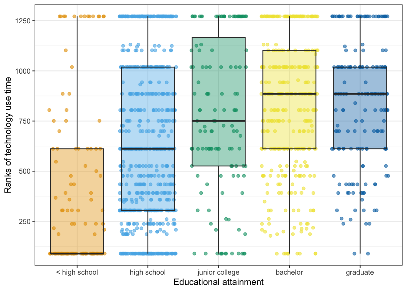
The graph confirms the result: The three college groups were very similar to one another, and there were differences among the other groups.
Eta-squared works for Kruskal-Wallis. (But didn’t we say in Section 7.7 that eta-squared has a positive bias and that we therefore should use omega-squared as outlined in Equation 7.4?)
Formula 7.5 : Computing eta-squared effect size
\[ \eta_{H}^2 = \frac{H-k+1}{n-k} \tag{7.6}\]
Besides a manual calculation I am going also to use {effectsize} and {lsr}.
Example 7.8 : Computation of eta-squared
R Code 7.41 : Computing eta-squared manually
#> [1] 0.0984431The value .098 is smaller than the omega-squared result of .11.
Assessment 7.2 : Interpretation of eta-squared effect size
The cutoff values are the same as for omega-squared:
A Kruskal-Wallis test found a statistically significant difference in technology use time at work across educational attainment groups (H = 142.21; p < .05). Based on a Dunn’s post hoc test, those with less than a high school education had statistically significantly lower mean ranked technology use time than all of the other groups (p < .05), and people with a bachelor’s degree, a graduate degree, or a junior college degree had significantly higher mean ranks than those with a high school diploma. There were no statistically significant differences among the three college groups. There was a medium effect size for the relationship between educational attainment and ranked values of technology use time (η2 = .098).
R Code 7.42 : Computing eta-squared with {effectsize}
effectsize::eta_squared(
    model = usetech_degree_aov
)
#> For one-way between subjects designs, partial eta squared is equivalent
#> to eta squared. Returning eta squared.#> # Effect Size for ANOVA
#>
#> Parameter | Eta2 | 95% CI
#> -------------------------------
#> DEGREE | 0.11 | [0.08, 1.00]
#>
#> - One-sided CIs: upper bound fixed at [1.00].This is the same result as with omega-squared!
R Code 7.43 : Computing eta-squared with {effectsize}
lsr::etaSquared(
    x = usetech_degree_aov
)
#> eta.sq eta.sq.part
#> DEGREE 0.1098235 0.1098235Example 7.9 : Time spent with technology at job by sex and educational attainment (degree)
R Code 7.44 : Boxplot: Percentage of time using technology at Work by sex
gss_2018_clean <- base::readRDS("data/chap07/gss_2018_clean.rds")

gss_2018_clean |>
    tidyr::drop_na(USETECH, SEX) |>
    dplyr::group_by(SEX) |>

    ggplot2::ggplot(
        ggplot2::aes(
            x = SEX,
            y = USETECH
        )
    ) +
    ggplot2::geom_boxplot(
        ggplot2::aes(
            fill = SEX
        ),
        alpha = .2
    ) +
    ggplot2::geom_jitter(
        ggplot2::aes(
            color = SEX
        ),
        alpha = 0.6
    ) +
    ggokabeito::scale_color_okabe_ito(guide = "none") +
    ggokabeito::scale_fill_okabe_ito(guide = "none") +
    ggplot2::labs(
        x = "Sex",
        y = "Percent of work time using technology"
    )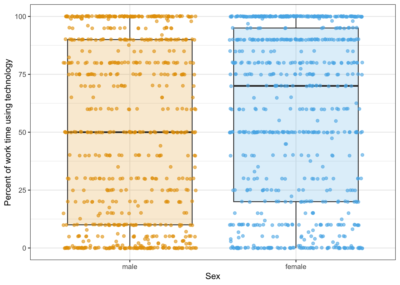
It seems that sex has some relationship to time spent on technology use.
R Code 7.45 : Boxplot: Percentage of time using technology at Work by sex & degree
gss_2018_clean |>
    tidyr::drop_na(USETECH, SEX, DEGREE) |>
    dplyr::group_by(SEX, DEGREE) |>

    ggplot2::ggplot(
        ggplot2::aes(
            x = DEGREE,
            y = USETECH
        )
    ) +
    ggplot2::geom_boxplot(
        ggplot2::aes(
            fill = SEX
        ),
        alpha = .2
    ) +

    ggokabeito::scale_color_okabe_ito(guide = "none") +
    ggokabeito::scale_fill_okabe_ito() +
    ggplot2::labs(
        x = "Educational attainment",
        y = "Percent of work time using technology"
    )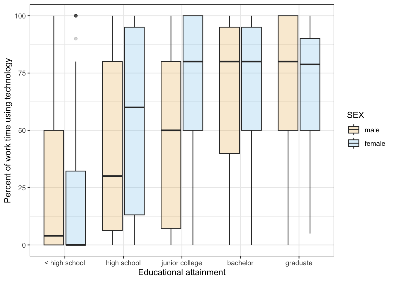
Males have higher use on technology only in the lowest educational achievement group (< high school.). In both highest groups (bachelor and graduate) males and females use technology at the job approximately at the same rate, whereas females with high school or junior college degree spend using technology at the job more time then males.
R Code 7.46 : Means plot of technology use at work by educational attainment and sex
gss_2018_clean |>
    tidyr::drop_na(USETECH) |>
    dplyr::group_by(DEGREE, SEX) |>
    dplyr::summarize(
        means = base::mean(USETECH),
        .groups = 'drop'
    ) |>

    ggplot2::ggplot(
        ggplot2::aes(
            x = DEGREE,
            y = means,
            group = SEX
        )
    ) +
    ggplot2::geom_point(
        ggplot2::aes(
            color = SEX
        ),
        size = 3
    ) +
    ggplot2::geom_line(
        ggplot2::aes(
            color = SEX
        ),
        linewidth = 1,
        linetype = "solid"
    ) +
    ggplot2::ylim(0, 100) +
    ggplot2::labs(
        x = "Educational attainment",
        y = "Percent of time spent using technology"
        ) +
    ggokabeito::scale_color_okabe_ito()
WATCH OUT! Using group in the aesthetic of the first layer
In this code chunk I have prepared the data.frame, e.g. calculated the means that I used for the graph. But then I needed inside the graph the equivalent of dplyr::group_by() as well. Normally the grouping is done implicitly but there are some common cases where the default does not work correctly:
group = 1.SEX grouping additionally to the display of USETECH by group means.(See for more detail the help file Aesthetics: grouping)
R Code 7.47 : Means plot of technology use at work by educational attainment and sex
gss_2018_clean |>
    ggplot2::ggplot(
        ggplot2::aes(
            x = DEGREE,
            y = USETECH,
            fill = SEX
            )
    ) +
    ggplot2::stat_summary(
        fun =  mean,
        geom = "point",
        size = 3,
        na.rm = TRUE,
        ggplot2::aes(
            color = SEX
        )
    ) +
    ggplot2::stat_summary(
        fun = mean,
        geom = "line",
        linewidth = 1,
        linetype = "solid",
        na.rm = TRUE,
        ggplot2::aes(
            group = SEX,
            color = SEX
        )
    ) +
    ggplot2::ylim(0, 100) +
    ggplot2::labs(
        x = "Educational attainment",
        y = "Percent of time spent using technology"
        ) +
    ggokabeito::scale_color_okabe_ito()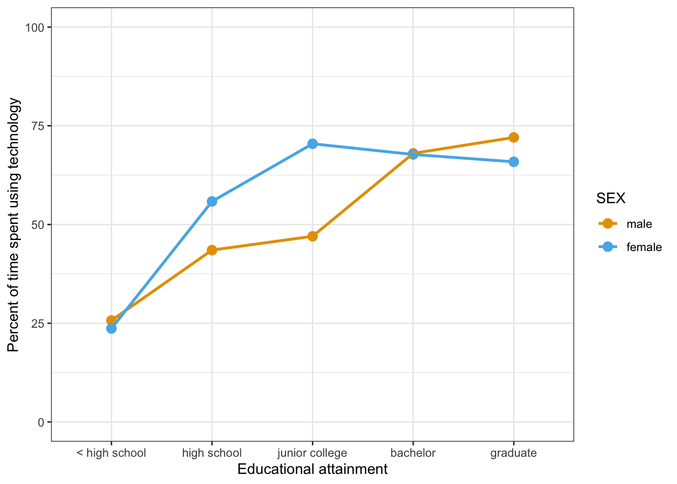
WATCH OUT! Using ggplot2::stat_summary()
I have still not much experience with ggplot2::stat_summary(). I used it the first time in R Code 3.64, but in that occasion I tried to prevent a warning message and applied in other respects the code provided by the book.
This time I used it for a group summary, e.g. a calculation I would have done with dplyr::group_by() and dplyr::summarize().
R Code 7.48 : Comparing means of technology use at work by educational attainment and sex
#> # A tibble: 10 × 4
#>    DEGREE         SEX    mean_usetech sd_usetech
#>    <fct>          <fct>         <dbl>      <dbl>
#>  1 < high school  male           25.7       35.4
#>  2 < high school  female         23.7       37.5
#>  3 high school    male           43.5       37.8
#>  4 high school    female         55.9       38.6
#>  5 junior college male           47.0       36.8
#>  6 junior college female         70.4       31.7
#>  7 bachelor       male           68.0       33.1
#>  8 bachelor       female         67.7       31.2
#>  9 graduate       male           72.1       29.2
#> 10 graduate       female         65.9       30.9
The biggest difference in time using technology at the job between male and female is in the group with a junior college degree.
But instead of using a visual calculation by head it is better to compute it in detail.
R Code 7.49 : Comparing means of technology use at work by educational attainment and sex
diff_sex_degree <- gss_2018_clean |>
  dplyr::group_by(DEGREE, SEX)  |>
  tidyr::drop_na(USETECH)  |>
  dplyr::summarize(
      mean_usetech = base::mean(USETECH),
      sd_usetech = stats::sd(USETECH),
      .groups = 'drop'
      ) |>
    dplyr::group_by(DEGREE) |>
    dplyr::summarize(diffs = diff(mean_usetech))

diff_means <- dplyr::full_join(
    x = mean_sd_usetech,
    y = diff_sex_degree,
    by = dplyr::join_by(DEGREE)
)

diff_means
#> # A tibble: 10 × 5
#> DEGREE SEX mean_usetech sd_usetech diffs
#> <fct> <fct> <dbl> <dbl> <dbl>
#> 1 < high school male 25.7 35.4 -2.04
#> 2 < high school female 23.7 37.5 -2.04
#> 3 high school male 43.5 37.8 12.3
#> 4 high school female 55.9 38.6 12.3
#> 5 junior college male 47.0 36.8 23.4
#> 6 junior college female 70.4 31.7 23.4
#> 7 bachelor male 68.0 33.1 -0.276
#> 8 bachelor female 67.7 31.2 -0.276
#> 9 graduate male 72.1 29.2 -6.17
#> 10 graduate female 65.9 30.9 -6.17The biggest difference in time using technology at the job between male and female is in the group with a junior college degree. The second biggest difference is only half of the first and happens in the high school group. Again about only half is the third difference in graduate, this time the sign is reversed.
These differences confirms quite well with Graph 7.15 and Graph 7.16.
Graph 7.15 and Graph 7.16 show that there interaction between the two variable SEX and DEGREE. because the lines are not parallel. Parallel lines would show that the mean of the continuous variable is consistently higher or lower for certain groups compared to others. Parallel lines indicate that there is no interaction between the two categorical variables.
But when the means plot — as in our example — shows lines that diverge or cross then there is an interaction between the categorical variables. The mean of the continuous variable is different at different levels of one categorical variable depending on the value of the other categorical variable. For example, mean technology use is lower for females compared to males for the lowest and highest educational attainment categories, but female technology use is higher than male technology use for the three other categories of educational attainment. The two variables are working together to influence the value of technology use.
Write the null and alternate hypotheses:
DEGREES and SEX.
DEGREES and SEX.
Compute the test statistic.
R Code 7.50 : Two-way ANOVA: Using technology by educational attainment and sex
#>               Df  Sum Sq Mean Sq F value   Pr(>F)
#> DEGREE         4  221301   55325  44.209  < 2e-16 ***
#> SEX            1   16473   16473  13.163 0.000296 ***
#> DEGREE:SEX     4   26510    6627   5.296 0.000311 ***
#> Residuals   1399 1750775    1251
#> ---
#> Signif. codes:  0 '***' 0.001 '**' 0.01 '*' 0.05 '.' 0.1 ' ' 1
#> 936 observations deleted due to missingness
There are three F-statistics for this ANOVA: one for each of the two individual variables (the main effects), and one for the interaction term.
When the interaction term is statistically significant, it is interpreted first and the main effects are only interpreted if a main effect variable influences the outcome alone.
Does a main effect variable influence the outcome alone?
SEX on USETECH without mentioning DEGREE than there was no main effect of SEX.Conclusion
There is no main effect variable that influences the outcome alone, therefore a repor contains only the interaction term.
Review and interpret the test statistics: Calculate the probability that your test statistic is at least as big as it is if there is no relationship (i.e., the null is true).
The p-value for the interaction term is with 0.000311 very tiny, and so the value of an F-statistic being as large or larger than the F-statistic for the interaction term happens a tiny percentage of the time when the null hypothesis is true.
Conclude and write report.
There was a statistically significant interaction between degree and sex on mean percent of work time spent using technology [F(4, 1399) = 5.3; p < .001]. The highest mean was 72.1% of time used for technology for males with graduate degrees. The lowest mean was 23.7% of the time for females with less than a high school diploma. The interaction between degree and sex shows that time spent on technology use increases more quickly for females, with both males and females eventually having high tech use in the top two educational attainment groups.
R Code 7.51 : Tukey’s HSD post hoc test for two-way ANOVA of USETECH by DEGREE and SEX
#>   Tukey multiple comparisons of means
#>     95% family-wise confidence level
#>
#> Fit: stats::aov(formula = USETECH ~ DEGREE * SEX, data = gss_2018_clean)
#>
#> $DEGREE
#>                                    diff       lwr       upr     p adj
#> high school-< high school    24.8247754 15.244768 34.404783 0.0000000
#> junior college-< high school 37.6070313 25.329478 49.884584 0.0000000
#> bachelor-< high school       43.0859568 32.760484 53.411429 0.0000000
#> graduate-< high school       43.9107249 32.376284 55.445165 0.0000000
#> junior college-high school   12.7822558  3.459487 22.105024 0.0017563
#> bachelor-high school         18.2611813 11.719691 24.802671 0.0000000
#> graduate-high school         19.0859494 10.766152 27.405746 0.0000000
#> bachelor-junior college       5.4789255 -4.608337 15.566188 0.5733923
#> graduate-junior college       6.3036936 -5.018002 17.625389 0.5490670
#> graduate-bachelor             0.8247681 -8.343540  9.993076 0.9991960
#>
#> $SEX
#>                diff      lwr      upr     p adj
#> female-male 6.80899 3.108699 10.50928 0.0003174
#>
#> $`DEGREE:SEX`
#>                                                   diff         lwr         upr
#> high school:male-< high school:male         17.8132060   2.7275183  32.8988937
#> junior college:male-< high school:male      21.3181818  -0.4992077  43.1355713
#> bachelor:male-< high school:male            42.3151914  25.7902764  58.8401064
#> graduate:male-< high school:male            46.3538961  27.5496712  65.1581210
#> < high school:female-< high school:male     -2.0378788 -22.6075109  18.5317533
#> high school:female-< high school:male       30.1500000  15.0344692  45.2655308
#> junior college:female-< high school:male    44.7418831  26.3028236  63.1809427
#> bachelor:female-< high school:male          42.0396406  25.8082011  58.2710800
#> graduate:female-< high school:male          40.1813241  22.0984520  58.2641962
#> junior college:male-high school:male         3.5049758 -14.4610385  21.4709901
#> bachelor:male-high school:male              24.5019854  13.5542915  35.4496792
#> graduate:male-high school:male              28.5406901  14.3851943  42.6961858
#> < high school:female-high school:male      -19.8510848 -36.2793820  -3.4227876
#> high school:female-high school:male         12.3367940   3.6616307  21.0119573
#> junior college:female-high school:male      26.9286771  13.2619985  40.5953557
#> bachelor:female-high school:male            24.2264346  13.7269673  34.7259018
#> graduate:female-high school:male            22.3681181   9.1859540  35.5502821
#> bachelor:male-junior college:male           20.9970096   1.8065820  40.1874372
#> graduate:male-junior college:male           25.0357143   3.8508477  46.2205808
#> < high school:female-junior college:male   -23.3560606 -46.1224714  -0.5896498
#> high school:female-junior college:male       8.8318182  -9.1592621  26.8228985
#> junior college:female-junior college:male   23.4237013   2.5622868  44.2851158
#> bachelor:female-junior college:male         20.7214588   1.7831557  39.6597618
#> graduate:female-junior college:male         18.8631423  -1.6841193  39.4104039
#> graduate:male-bachelor:male                  4.0387047 -11.6416301  19.7190396
#> < high school:female-bachelor:male         -44.3530702 -62.1121183 -26.5940220
#> high school:female-bachelor:male           -12.1651914 -23.1539720  -1.1764108
#> junior college:female-bachelor:male          2.4266917 -12.8138117  17.6671952
#> bachelor:female-bachelor:male               -0.2755508 -12.7548798  12.2037783
#> graduate:female-bachelor:male               -2.1338673 -16.9414427  12.6737082
#> < high school:female-graduate:male         -48.3917749 -68.2892584 -28.4942914
#> high school:female-graduate:male           -16.2038961 -30.3911918  -2.0166004
#> junior college:female-graduate:male         -1.6120130 -19.2981376  16.0741116
#> bachelor:female-graduate:male               -4.3142555 -19.6849976  11.0564866
#> graduate:female-graduate:male               -6.1725720 -23.4870269  11.1418829
#> high school:female-< high school:female     32.1878788  15.7321731  48.6435845
#> junior college:female-< high school:female  46.7797619  27.2270154  66.3325084
#> bachelor:female-< high school:female        44.0775194  26.5912218  61.5638170
#> graduate:female-< high school:female        42.2192029  23.0019908  61.4364150
#> junior college:female-high school:female    14.5918831   0.8922699  28.2914963
#> bachelor:female-high school:female          11.8896406   1.3473395  22.4319416
#> graduate:female-high school:female          10.0313241  -3.1849820  23.2476303
#> bachelor:female-junior college:female       -2.7022425 -17.6240305  12.2195454
#> graduate:female-junior college:female       -4.5605590 -21.4777217  12.3566037
#> graduate:female-bachelor:female             -1.8583165 -16.3376501  12.6210171
#>                                                p adj
#> high school:male-< high school:male        0.0072699
#> junior college:male-< high school:male     0.0619111
#> bachelor:male-< high school:male           0.0000000
#> graduate:male-< high school:male           0.0000000
#> < high school:female-< high school:male    0.9999995
#> high school:female-< high school:male      0.0000000
#> junior college:female-< high school:male   0.0000000
#> bachelor:female-< high school:male         0.0000000
#> graduate:female-< high school:male         0.0000000
#> junior college:male-high school:male       0.9998264
#> bachelor:male-high school:male             0.0000000
#> graduate:male-high school:male             0.0000000
#> < high school:female-high school:male      0.0052315
#> high school:female-high school:male        0.0003049
#> junior college:female-high school:male     0.0000000
#> bachelor:female-high school:male           0.0000000
#> graduate:female-high school:male           0.0000039
#> bachelor:male-junior college:male          0.0192892
#> graduate:male-junior college:male          0.0071871
#> < high school:female-junior college:male   0.0389231
#> high school:female-junior college:male     0.8690307
#> junior college:female-junior college:male  0.0141081
#> bachelor:female-junior college:male        0.0192858
#> graduate:female-junior college:male        0.1039186
#> graduate:male-bachelor:male                0.9983501
#> < high school:female-bachelor:male         0.0000000
#> high school:female-bachelor:male           0.0167764
#> junior college:female-bachelor:male        0.9999688
#> bachelor:female-bachelor:male              1.0000000
#> graduate:female-bachelor:male              0.9999867
#> < high school:female-graduate:male         0.0000000
#> high school:female-graduate:male           0.0113631
#> junior college:female-graduate:male        0.9999998
#> bachelor:female-graduate:male              0.9967894
#> graduate:female-graduate:male              0.9816675
#> high school:female-< high school:female    0.0000000
#> junior college:female-< high school:female 0.0000000
#> bachelor:female-< high school:female       0.0000000
#> graduate:female-< high school:female       0.0000000
#> junior college:female-high school:female   0.0261888
#> bachelor:female-high school:female         0.0133486
#> graduate:female-high school:female         0.3233313
#> bachelor:female-junior college:female      0.9999069
#> graduate:female-junior college:female      0.9976459
#> graduate:female-bachelor:female 0.9999951$DEGREE was comparing groups of DEGREE to each other.$SEX was comparing males and females to each other.DEGREE*SEX with each other.
This indicates that there is a statistically significant (p < .05) difference of 17.81 between the mean percentage time of technology use for males with less than high school compared to males with high school in the sample, and that the difference between the mean of these two groups is likely somewhere between 2.73 and 32.90 in the population this sample came from.
There are so many groups with significant differences that it would be more useful to just include the boxplot from the exploratory analysis or the means plot of Graph 7.15 and a paragraph about any interesting overall patterns in the comparisons. For instance:
There is a trend that with higher educational attainment the time spent with technology at work grows. Starting from the same relatively low level of 25% the use of technology with higher degrees rises faster for female than for males until the junior college degree. In the following higher educational attainment groups (bachelor and graduate) the time used with technology decreases for females whereas it continues to increase for males. Both trends cross at the bachelor level with about 68% and reach 66% for female and 72% for males at the graduate level.
The biggest difference in time using technology at the job between male and female is in the group with a junior college degree (junior college:female-junior college:male).
The second biggest difference is only half of the first and happens in the high school group (high school:female-< high school:male).
All the other differences between female and males at the same degree level are not statistically significant with p <= .05.
Testing the normality assumption is more difficult as with the one-way ANOVA, we would need to look at each group. Since there are five degree groups, two sex groups, and 10 degree-by-sex groups (e.g., male and less than high school). Instead of checking normality one group at a time when there are a large number of groups in an ANOVA model, this assumption can be checked by examining the residuals. The residuals are the distances between the value of the outcome for each person and the value of the group mean for that person. When the residuals are normally distributed, this indicates that the values in each group are normally distributed around the group mean.
Example 7.10 : Testing normality for two-way ANOVA
R Code 7.52 : Shapiro-Wilk test for normal distribution by groups
stats::shapiro.test(
    aov_test <- stats::aov(
    formula = USETECH ~ DEGREE * SEX,
    data = gss_2018_clean
    )$residuals
)
#>
#> Shapiro-Wilk normality test
#>
#> data: aov_test <- stats::aov(formula = USETECH ~ DEGREE * SEX, data = gss_2018_clean)$residuals
#> W = 0.95984, p-value < 2.2e-16Instead of providing the result of the model fitting with the stats::aov() function I have nested the function into the Shapiro-Wilk test. The statistically significant p-value means that we have to reject the null hypotheses (“The distribution is normal”). So, this test shows that the residuals fail the normality assumption.
To confirm the result it is helpful to graph the residuals.
R Code 7.53 : Inspecting normality with a graph of the residuals
aov_residuals_df <- tibble::tibble(residuals =
        stats::aov(
        formula = USETECH ~ DEGREE * SEX,
        data = gss_2018_clean
        )$residuals
    )

p1 <- my_hist_dnorm(
    df = aov_residuals_df,
    v = aov_residuals_df$residuals,
    n_bins = 30,
    x_label = "Residuals with 30 bins as in the book")

p2 <- my_hist_dnorm(
    df = aov_residuals_df,
    v = aov_residuals_df$residuals,
    n_bins = 20,
    x_label = "Residuals with 20 bins")

gridExtra::grid.arrange(
    p1, p2,
    nrow = 2
)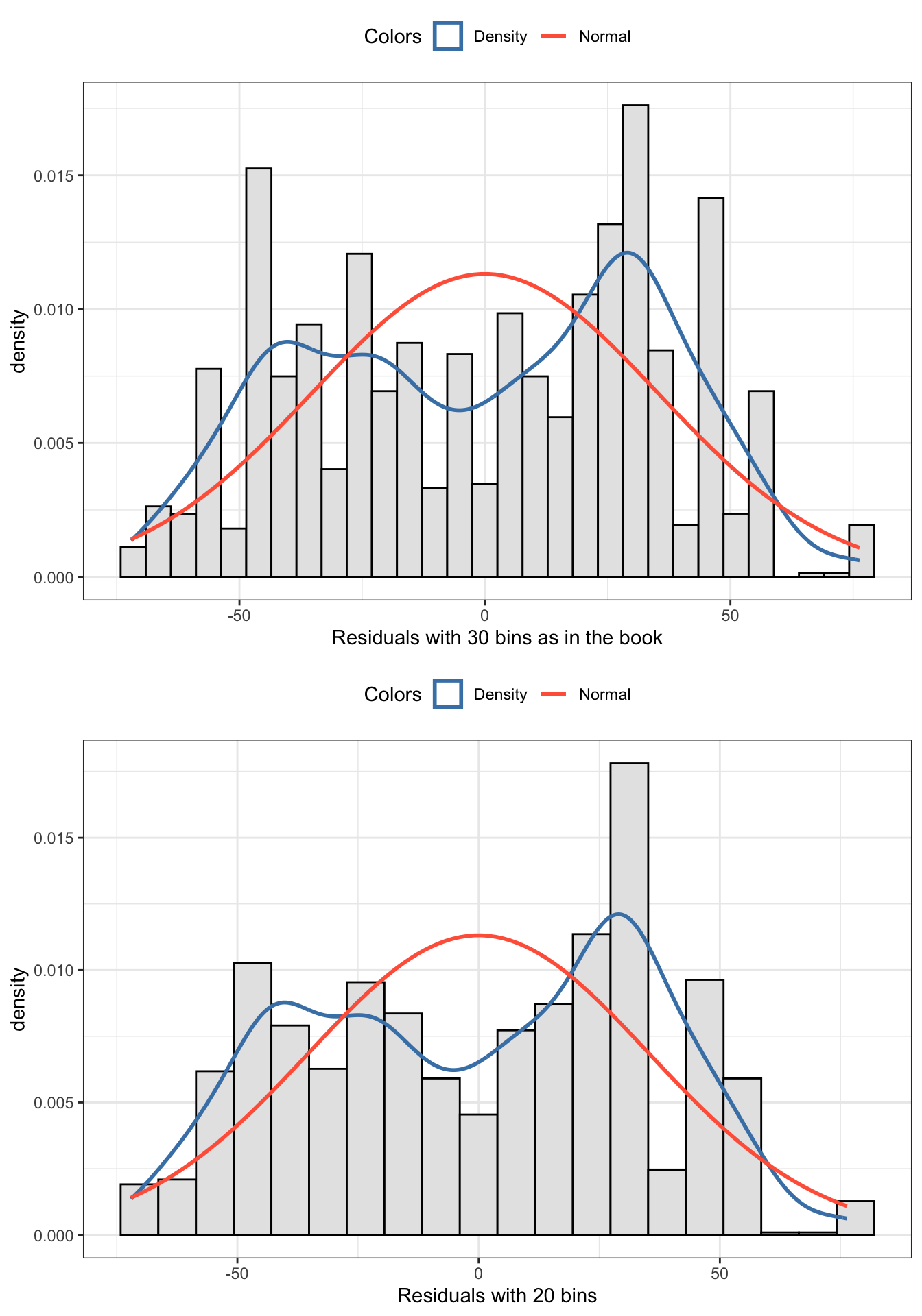
The graph is clearly not normal. The insinuated bi-modality in the text of the book is in my opinion an artifact of the chosen number of bins. To compare I have graphed two histograms with 30 and 20 bins.
R Code 7.54 : Levene’s test for two-way ANOVA
glue::glue("############### default: `center = mean` ####################")
car::leveneTest(
    y = USETECH ~ DEGREE * SEX,
    center = mean,
    data = gss_2018_clean
)

glue::glue(" ")
glue::glue("############### default: `center = median` #################")
car::leveneTest(
    y = USETECH ~ DEGREE * SEX,
    center = median,
    data = gss_2018_clean
)
#> ############### default: `center = mean` ####################
#> Levene's Test for Homogeneity of Variance (center = mean)
#> Df F value Pr(>F)
#> group 9 8.5912 1.289e-12 ***
#> 1399
#> ---
#> Signif. codes: 0 '***' 0.001 '**' 0.01 '*' 0.05 '.' 0.1 ' ' 1
#>
#> ############### default: `center = median` #################
#> Levene's Test for Homogeneity of Variance (center = median)
#> Df F value Pr(>F)
#> group 9 7.1573 3.324e-10 ***
#> 1399
#> ---
#> Signif. codes: 0 '***' 0.001 '**' 0.01 '*' 0.05 '.' 0.1 ' ' 1WATCH OUT! What is the center of each group?
Using the means at the center is the original test. The default center = median provides a more robust test. But even this more robust test is also statistically significant. So the homogeneity of variance has to be rejected in both cases.
The results were statistically significant so the null hypothesis was rejected in this test as well. The equal variances assumption was not met.
The two-way ANOVA had failed its assumptions.
The books mentions stats::friedman.test(). But it turns out that the test result is not statistically significant. This seems unlikely given all the other information we have about the data distribution.
We had already computed the ranks of USETECH for the Dunn’s test earlier in Example 7.7. We can load the appropriate gss_2018_clean3.rds data and use the variable usetech_rank.
R Code 7.55 : Two-way ANOVA ranked technology use by degree and sex
#>               Df    Sum Sq Mean Sq F value   Pr(>F)
#> DEGREE         4  23270305 5817576   40.26  < 2e-16 ***
#> SEX            1   1849104 1849104   12.80 0.000359 ***
#> DEGREE:SEX     4   3120976  780244    5.40 0.000258 ***
#> Residuals   1399 202148767  144495
#> ---
#> Signif. codes:  0 '***' 0.001 '**' 0.01 '*' 0.05 '.' 0.1 ' ' 1
#> 936 observations deleted due to missingnessA two-way ANOVA with ranked technology time use as the outcome found a statistically significant interaction between degree and sex (p < .05). The overall pattern of results indicates that males and females with less than a high school education use technology the least, while those with higher educational attainment use technology the most. Males and females differ a lot in use of technology for those with a junior college degree, with females having a junior college degree having the highest use of technology of all females.
WATCH OUT! What’s the difference between ranked and not ranked?
I have to confess that I do not understand the difference between our (wrong?) tests with assuming that the normality and homogeneity of variance assumptions hold and here now the ranked version of the two-way ANOVA. It seems to me that the results are the same. Even the both graphs are almost identical.
Another suggestion for alternative test is the Box-Cox transformation on the outcome variable. The Box-Cox power transformations were developed to reduce the non-normality of residuals, so they might be useful here. The original paper by Box and Cox explains the transformations (Box and Cox 1964), and there are numerous tutorials on the use of them (Wikipedia 2021; Zach 2020; Glen, n.d.; Lane 2017).
| term | definition |
|---|---|
| ANOVA | Analysis of variance is a statistical method used to compare means across groups to determine whether there is a statistically significant difference among the means; typically used when there are three or more means to compare. (SwR, Glossary) |
| Bonferroni | Bonferroni post hoc test is a pairwise test used after a statistically significant ANOVA that conducts a t-test for each pair of means but adjusts the threshold for statistical significance to ensure that there is a small enough risk of Type I error; it is generally considered a very conservative post hoc test that only identifies the largest differences between means as statistically significant. (SwR, Glossary) |
| Brown-Forsythe | Brown-Forsythe is an alternate F-statistic used for analysis of variance when the assumption of homogeneity of variance is not met; the Brown-Forsythe F-statistic is computed after transforming the values of the outcome to represent the distance from the median. (SwR, Glossary) |
| Ceiling | A ceiling effect happens when many observations are at the highest possible value for a variable. (SwR, Glossary) |
| Chi-squared | Chi-squared is the test statistic following the chi-squared probability distribution; the chi-squared test statistic is used in inferential tests, including examining the association between two categorical variables and determining statistical significance for a logistic regression model. (SwR, Glossary) |
| Cohen’s d | Cohen’s d is a standardized effect size for measuring the difference between two group means. It is frequently used to compare a treatment to a control group. It can be a suitable effect size to include with t-test and ANOVA results. (<a href= "https://statisticsbyjim.com/basics/cohens-d/">Statistics by Jim</a>) |
| Contrasts | Contrasts are sets of numbers used in planned contrasts to specify which means or groups of means to compare to each other, usually to identify statistically significant differences among means after a statistically significant analysis of variance. (SwR, Glossary) |
| Cramér’s V | Cramér’s V is an effect size to determine the strength of the relationship between two categorical variables; often reported with the results of a chi-squared. (SwR, Glossary) |
| CVD | Color vision deficiency (CVD) or color blindness (also spelled colour blindness) includes a wide range of causes and conditions and is actually quite complex. It's a condition characterized by an inability or difficulty in perceiving and differentiating certain colors due to abnormalities in the three color-sensing pigments of the cones in the retina. (<a href="https://enchroma.com/pages/types-of-color-blindness">EnChroma</a>) |
| Degrees of Freedom | Degree of Freedom (df) is the number of pieces of information that are allowed to vary in computing a statistic before the remaining pieces of information are known; degrees of freedom are often used as parameters for distributions (e.g., chi-squared, F). (SwR, Glossary) |
| Dunn | Dunn’s post hoc test is a pairwise comparisons to determine which groups are statistically significantly different from one another following a significant [Kruskal-Wallis] test. (SwR, Glossary) |
| Effect Size | Effect size is a measure of the strength of a relationship; effect sizes are important in inferential statistics in order to determine and communicate whether a statistically significant result has practical importance. (SwR, Glossary) |
| Eta-squared | Eta-squared is an [effect size] interpreted as the proportion of variability in the continuous outcome variable that is explained by groups in an analysis of variance; recent research suggests that eta-squared is biased and that [omega-squared] may be a less biased alternative following analysis of variance. (SwR, Glossary) |
| F-Statistic | F-statistic is a test statistic comparing explained and unexplained variance in [ANOVA] and linear regression. The F-statistic is a ratio where the variation between the groups is compared to the variation within the groups. (SwR, Glossary) |
| Familywise | Familywise error is the alpha or Type I error rate when conducting multiple statistical tests. A large familywise alpha is one of the reasons that analysis of variance is preferable to conducting multiple t-tests when comparing means across more than two groups. (SwR, Glossary) |
| Floor | A floor effect happens when a variable has many observations that take the lowest value of the variable, which can indicate that the range of values was insufficient to capture the true variability of the data. (SwR, Glossary) |
| Grand | Grand mean is the overall mean of a continuous variable that is used to determine distances from the mean for individuals and groups in ANOVA. (SwR, Glossary) |
| HSD | Tukey’s Honestly Significant Difference (HSD) is a post hoc test to determine which means are statistically significantly different from each other following a significant ANOVA result; Tukey’s HSD compares each pair of means and so is considered a pairwise test, but it is less conservative than the Bonferroni post hoc test. (SwR, Glossary) |
| Kruskal-Wallis | Kruskal-Wallis test is used to compare ranks across three or more groups when the normal distribution assumption fails for analysis of variance (ANOVA) (SwR, Glossary) |
| Kurtosis | Kurtosis is a measure of how many observations are in the tails of a distribution; distributions that look bell-shaped, but have a lot of observations in the tails (platykurtic) or very few observations in the tails (leptokurtic) (SwR, Glossary) |
| Levene | Levene’s test is a statistical test to determine whether observed data meet the homogeneity of variances assumption; Levene’s test is used to test this assumption for t-tests and analysis of variance. (SwR, Glossary) |
| Main Effect | Main effect is the relationship between only one of the independent variables and the dependent variable, ignoring the impact of any additional independent variables or interaction effects. (SwR, Glossary) |
| Odds Ratio | Odds is usually defined in statistics as the probability an event will occur divided by the probability that it will not occur. An odds ratio (OR) is a measure of association between a certain property A and a second property B in a population. Specifically, it tells you how the presence or absence of property A has an effect on the presence or absence of property B. (<a href="https://www.statisticshowto.com/probability-and-statistics/probability-main-index/odds-ratio/">Statistics How To</a>). An odds ratio is a ratio of two ratios. They quantify the strength of the relationship between two conditions. They indicate how likely an outcome is to occur in one context relative to another. (<a href="https://statisticsbyjim.com/probability/odds-ratio/">Statistics by Jim</a>) |
| Omega-squared | Omega-squared is an effect size for determining the strength of a relationship following an analysis of variance ([ANOVA]) statistical test. In contrast to [eta-squared] it is adjusted to account for the positive bias, and is more stable when assumptions are not completely met. (SwR, Glossary) |
| Omnibus | An omnibus is a statistical test that identifies that there is some relationship going on between variables, but not what that relationship is. (SwR, Glossary) |
| p-hacking | P-hacking is a set of statistical decisions and methodology choices during research that artificially produces statistically significant results. These decisions increase the probability of false positives—where the study indicates an effect exists when it actually does not. P-hacking is also known as data dredging, data fishing, and data snooping. (<a href="https://statisticsbyjim.com/hypothesis-testing/p-hacking/">Statistics by Jim</a>) |
| p-value | The p-value is the probability that the test statistic is at least as big as it is under the null hypothesis (SwR, Glossary) |
| Pairwise Comparisons | Pairwise comparisons are comparisons between every pair of groups to identify which are statistically significantly different from one another following a statistically significant result in an analysis of variance (ANOVA) or other multigroup analysis. (SwR, Glossary) |
| Planned Comparisons | Planned comparisons is a statistical strategy for comparing different groups, often used after a statistically significant analysis of variance to test hypotheses about which group means are statistically significantly different from one another. (SwR, Glossary) |
| Platykurtic | Platykurtic is a distribution of a numeric variable that has more observations in the tails than a normal distribution would have; platykurtic distributions often look flatter than a normal distribution. (SwR, Glossary) |
| Residually | Residuals are the differences between the observed values and the predicted values. (SwR, Glossary) |
| Shapiro-Wilk | The Shapiro-Wilk test is a statistical test to determine or confirm whether a variable has a normal distribution; it is sensitive to small deviations from normality and not useful for sample sizes above 5,000 because it will nearly always find non-normality. (SwR, Glossary) |
| Standardized Residuals | Standardized residuals are the standardized differences between observed and expected values in a chi-squared analysis; a large standardized residual indicates that the observed and expected values were very different. (SwR, Glossary) |
| Student | Student t-test is a statistical test used to test whether the difference between the response of two groups is statistically significant or not. (<a href="https://en.wikipedia.org/wiki/Student%27s_t-test">Wikipedia</a>) |
| T-Test | A t-test is a type of statistical analysis used to compare the averages of two groups and determine whether the differences between them are more likely to arise from random chance. (<a href="https://en.wikipedia.org/wiki/Student%27s_t-test">Wikipedia</a>) |
| Tukey | Tukey’s Honestly Significant Difference (HSD) is a post hoc test to determine which means are statistically significantly different from each other following a significant ANOVA result; Tukey’s HSD compares each pair of means and so is considered a pairwise test, but it is less conservative than the [Bonferroni] post hoc test. (SwR, Glossary) |
| Type-1 | Rejecting the null hypothesis when it should be retained is called Type I error or alpha and used as the threshold to determine statistical significance. (SwR, Glossary) |
| Type-2 | Retaining the null hypothesis when it should be rejected is calles Type II error or beta. (SwR, Glossary) |
Session Info
sessioninfo::session_info()#> ─ Session info ───────────────────────────────────────────────────────────────
#> setting value
#> version R version 4.4.2 (2024-10-31)
#> os macOS Sequoia 15.1
#> system x86_64, darwin20
#> ui X11
#> language (EN)
#> collate en_US.UTF-8
#> ctype en_US.UTF-8
#> tz Europe/Vienna
#> date 2024-11-13
#> pandoc 3.5 @ /usr/local/bin/ (via rmarkdown)
#>
#> ─ Packages ───────────────────────────────────────────────────────────────────
#> package * version date (UTC) lib source
#> abind 1.4-8 2024-09-12 [2] CRAN (R 4.4.1)
#> bayestestR 0.15.0 2024-10-17 [2] CRAN (R 4.4.1)
#> car 3.1-3 2024-09-27 [2] CRAN (R 4.4.1)
#> carData 3.0-5 2022-01-06 [2] CRAN (R 4.4.0)
#> cli 3.6.3 2024-06-21 [2] CRAN (R 4.4.1)
#> coda 0.19-4.1 2024-01-31 [2] CRAN (R 4.4.0)
#> codetools 0.2-20 2024-03-31 [2] CRAN (R 4.4.2)
#> colorblindr 0.1.0 2024-04-25 [2] Github (clauswilke/colorblindr@90d64f8)
#> colorspace 2.1-1 2024-07-26 [2] CRAN (R 4.4.0)
#> commonmark 1.9.2 2024-10-04 [2] CRAN (R 4.4.1)
#> cowplot 1.1.3.9000 2024-04-25 [2] Github (wilkelab/cowplot@e1334a2)
#> crayon 1.5.3 2024-06-20 [2] CRAN (R 4.4.0)
#> curl 6.0.0 2024-11-05 [2] CRAN (R 4.4.1)
#> datawizard 0.13.0 2024-10-05 [2] CRAN (R 4.4.1)
#> digest 0.6.37 2024-08-19 [2] CRAN (R 4.4.1)
#> dplyr 1.1.4 2023-11-17 [2] CRAN (R 4.4.0)
#> dunn.test 1.3.6 2024-04-12 [2] CRAN (R 4.4.0)
#> effectsize 0.8.9 2024-07-03 [2] CRAN (R 4.4.0)
#> emmeans 1.10.5 2024-10-14 [2] CRAN (R 4.4.1)
#> estimability 1.5.1 2024-05-12 [2] CRAN (R 4.4.0)
#> evaluate 1.0.1 2024-10-10 [2] CRAN (R 4.4.1)
#> fansi 1.0.6 2023-12-08 [2] CRAN (R 4.4.0)
#> farver 2.1.2 2024-05-13 [2] CRAN (R 4.4.0)
#> fastmap 1.2.0 2024-05-15 [2] CRAN (R 4.4.0)
#> forcats 1.0.0 2023-01-29 [2] CRAN (R 4.4.0)
#> Formula 1.2-5 2023-02-24 [2] CRAN (R 4.4.0)
#> generics 0.1.3 2022-07-05 [2] CRAN (R 4.4.0)
#> ggokabeito 0.1.0 2021-10-18 [2] CRAN (R 4.4.0)
#> ggplot2 3.5.1 2024-04-23 [2] CRAN (R 4.4.0)
#> glossary * 1.0.0.9003 2024-08-05 [2] Github (debruine/glossary@05e4a61)
#> glue 1.8.0 2024-09-30 [2] CRAN (R 4.4.1)
#> gridExtra 2.3 2017-09-09 [2] CRAN (R 4.4.0)
#> gtable 0.3.6 2024-10-25 [2] CRAN (R 4.4.1)
#> here 1.0.1 2020-12-13 [2] CRAN (R 4.4.0)
#> htmltools 0.5.8.1 2024-04-04 [2] CRAN (R 4.4.0)
#> htmlwidgets 1.6.4 2023-12-06 [2] CRAN (R 4.4.0)
#> insight 0.20.5 2024-10-02 [2] CRAN (R 4.4.1)
#> jsonlite 1.8.9 2024-09-20 [2] CRAN (R 4.4.1)
#> kableExtra 1.4.0 2024-01-24 [2] CRAN (R 4.4.0)
#> knitr 1.49 2024-11-08 [2] CRAN (R 4.4.1)
#> labeling 0.4.3 2023-08-29 [2] CRAN (R 4.4.0)
#> lattice 0.22-6 2024-03-20 [2] CRAN (R 4.4.2)
#> lifecycle 1.0.4 2023-11-07 [2] CRAN (R 4.4.0)
#> lsr 0.5.2 2021-12-01 [2] CRAN (R 4.4.0)
#> magrittr 2.0.3 2022-03-30 [2] CRAN (R 4.4.0)
#> markdown 1.13 2024-06-04 [2] CRAN (R 4.4.0)
#> MASS 7.3-61 2024-06-13 [2] CRAN (R 4.4.2)
#> Matrix 1.7-1 2024-10-18 [2] CRAN (R 4.4.2)
#> moments 0.14.1 2022-05-02 [2] CRAN (R 4.4.0)
#> multcomp 1.4-26 2024-07-18 [2] CRAN (R 4.4.0)
#> munsell 0.5.1 2024-04-01 [2] CRAN (R 4.4.0)
#> mvtnorm 1.3-2 2024-11-04 [2] CRAN (R 4.4.1)
#> nortest 1.0-4 2015-07-30 [2] CRAN (R 4.4.0)
#> onewaytests 3.0 2023-10-01 [2] CRAN (R 4.4.0)
#> parameters 0.23.0 2024-10-18 [2] CRAN (R 4.4.1)
#> pillar 1.9.0 2023-03-22 [2] CRAN (R 4.4.0)
#> pkgconfig 2.0.3 2019-09-22 [2] CRAN (R 4.4.0)
#> purrr 1.0.2 2023-08-10 [2] CRAN (R 4.4.0)
#> R6 2.5.1 2021-08-19 [2] CRAN (R 4.4.0)
#> RColorBrewer 1.1-3 2022-04-03 [2] CRAN (R 4.4.0)
#> rlang 1.1.4 2024-06-04 [2] CRAN (R 4.4.0)
#> rmarkdown 2.29 2024-11-04 [2] CRAN (R 4.4.1)
#> rprojroot 2.0.4 2023-11-05 [2] CRAN (R 4.4.0)
#> rstudioapi 0.17.1 2024-10-22 [2] CRAN (R 4.4.1)
#> rversions 2.1.2 2022-08-31 [2] CRAN (R 4.4.0)
#> sandwich 3.1-1 2024-09-15 [2] CRAN (R 4.4.1)
#> scales 1.3.0 2023-11-28 [2] CRAN (R 4.4.0)
#> sessioninfo 1.2.2 2021-12-06 [2] CRAN (R 4.4.0)
#> stringi 1.8.4 2024-05-06 [2] CRAN (R 4.4.0)
#> stringr 1.5.1 2023-11-14 [2] CRAN (R 4.4.0)
#> survival 3.7-0 2024-06-05 [2] CRAN (R 4.4.2)
#> svglite 2.1.3 2023-12-08 [2] CRAN (R 4.4.0)
#> systemfonts 1.1.0 2024-05-15 [2] CRAN (R 4.4.0)
#> TH.data 1.1-2 2023-04-17 [2] CRAN (R 4.4.0)
#> tibble 3.2.1 2023-03-20 [2] CRAN (R 4.4.0)
#> tidyr 1.3.1 2024-01-24 [2] CRAN (R 4.4.0)
#> tidyselect 1.2.1 2024-03-11 [2] CRAN (R 4.4.0)
#> utf8 1.2.4 2023-10-22 [2] CRAN (R 4.4.0)
#> vctrs 0.6.5 2023-12-01 [2] CRAN (R 4.4.0)
#> viridisLite 0.4.2 2023-05-02 [2] CRAN (R 4.4.0)
#> wesanderson 0.3.7 2023-10-31 [2] CRAN (R 4.4.0)
#> withr 3.0.2 2024-10-28 [2] CRAN (R 4.4.1)
#> xfun 0.49 2024-10-31 [2] CRAN (R 4.4.1)
#> xml2 1.3.6 2023-12-04 [2] CRAN (R 4.4.0)
#> xtable 1.8-4 2019-04-21 [2] CRAN (R 4.4.0)
#> yaml 2.3.10 2024-07-26 [2] CRAN (R 4.4.0)
#> zoo 1.8-12 2023-04-13 [2] CRAN (R 4.4.0)
#>
#> [1] /Library/Frameworks/R.framework/Versions/4.4-x86_64/library
#> [2] /Library/Frameworks/R.framework/Versions/4.4-x86_64/Resources/library
#>
#> ──────────────────────────────────────────────────────────────────────────────