Achievement 1: (Understanding variable types and data types) (Section 2.4). As I already know this information I will skip this achievement. This empty section is only mentioned to get the same section numbering as in the book.
Achievement 2: Choosing and conducting descriptive analyses for categorical (factor) variables (Section 2.5)
Achievement 3: Choosing and conducting descriptive analyses for continuous (numeric) variables (Section 2.6)
Subject of this chapter is the transgender health care problem.
Transgender people are people whose biological sex is not consistent with their gender.
Cisgender people are people whose gender identity matches their biological sex.
In this chapter we are going to use data from the BRFSS website. The Behavioral Risk Factor Surveillance System (BRFSS) is a system of health-related telephone surveys that collect state data about U.S. residents regarding their health-related risk behaviors, chronic health conditions, and use of preventive services. Established in 1984 with 15 states, BRFSS now collects data in all 50 states as well as the District of Columbia and three U.S. territories. BRFSS completes more than 400,000 adult interviews each year, making it the largest continuously conducted health survey system in the world. (BRFSS)
The rationale of this chapter is the fact, that prior to examining statistical relationships among variables, published studies in academic journals usually present descriptive statistics. What kind of measures exist and how to describe the data set is an important task before one can start to analyse statistical relations. The following screenshot from (Narayan, Lebron-Zapata, and Morris 2017, 876) demonstrates how such descriptive statistics can be summarized to create a so-called Table 1 as an introduction to the subject:
Graph 2.1: Screenshot of Table 1, “Transgender Survey Participants Demographics” from Narayan et. al. (2017)
In this chapter we are going to reproduce Graph 2.1 and add some additional information.
2.3 Data, codebook, and R packages
Resource 2.1 : Data, codebook, and R packages for learning about descriptive statistics
To know about variable and data types is essential as different types require different approaches for the analysis.
The following outline of the next sections is slightly adapted from the book. Harris has some measures of categorical variables (mode and index of qualitative variation) explained in the section on numeric variables.
Categorical variables:
Central tendency: The two most commonly used and reported descriptive statistics for categorical (or factor) data types are frequencies and percentages. Sometimes also the mode is used to identify the most common (or typical) category of a factor variable.
Spread / Variety: is for for categorical variables not often reported. Harris mentions the index of qualitative variation, which quantifies how much the observations are spread across the categories of a categorical variable.
Numerical variables:
Central tendency: The most important measures are the mean, median and mode.
For the decision if one should report mean or median in numerical variables the measures for skewness and kurtosis are helpful. Another issue with numerical variables is usage of scientific notation.
I will explain explicitly only to those subjects where I am not firm. This is
Bullet List 2.1: Subjects reviewed in this chapter
But I will address all the other measures in the examples resp. exercises.
2.4.2 Get the data
But before we are going to work with the data we have do download it form the BRFSS website.
Watch out!
Downloading the huge file (69 MB as ZIP and 1 GB unzipped) will take some minutes. So be patient!
R Code 2.1 : Download the SAS transport file data from the BRFSS website and save dataframe with selected variables as R object
Code
## run this code chunk only once (manually)url<-"http://www.cdc.gov/brfss/annual_data/2014/files/LLCP2014XPT.zip"utils::download.file( url =url, destfile =tf<-base::tempfile(), mode ="wb")brfss_2014<-haven::read_xpt(tf)brfss_tg_2014<-brfss_2014|>dplyr::select(TRNSGNDR, `_AGEG5YR`, `_RACE`, `_INCOMG`, `_EDUCAG`, HLTHPLN1, HADMAM, `_AGE80`, PHYSHLTH)data_folder<-base::paste0(here::here(), "/data/")if(!base::file.exists(data_folder)){base::dir.create(data_folder)}chap02_folder<-base::paste0(here::here(), "/data/chap02/")if(!base::file.exists(chap02_folder)){base::dir.create(chap02_folder)}base::saveRDS(object =brfss_tg_2014, file =paste0(chap02_folder, "/brfss_tg_2014_raw.rds"))
Listing / Output 2.1: Download and save the transgender data 2014 from the BRFSS website
The original file has 279 variables and 464664 observations. After selecting only 9 variable the file is with 31.9 MB (memory usage) and stored compressed (2.2 MB) much smaller.
Four observations about the code
It is not possible to download the file with haven::read_xpt(<URL>) directly. At first one has to create a temporary file to store the zipped file.
Whenever you meet a variable / row name with a forbidden R syntax surround the name with backticks (grave accents).
Instead of exporting the R object into a .csv file I save the data as a compressed R object that can loaded easily again into the computer memory with the base::readRDS() function.
With regard to the base::saveRDS() function I have to remind myself that the first argument is the R object without quotes. I committed this error several times.
2.5 Descriptive analyses for categorical (factor) variables
The goal of this section is to summarize and interpret the categorical variable TRNSGNDR. In contrast to the book I will work with a dataframe consisting only of the variable which I will recode to transgender.
2.5.1 Summarize categorical variables without recoding
Example 2.1 : Summarize categorical variables without recoding
Listing / Output 2.2: Show structure of the transgender data with utils::str()
#> tibble [464,664 × 1] (S3: tbl_df/tbl/data.frame)
#>  $ TRNSGNDR: num [1:464664] NA NA NA NA NA NA NA NA NA NA ...
#>   ..- attr(*, "label")= chr "DO YOU CONSIDER YOURSELF TO BE TRANSGEND"
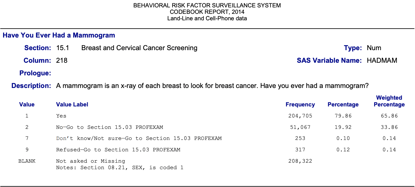
{haven} has imported labelled data for the variables. We can use these labels to find the appropriate passages in the 126 pages of the codebook. Just copy the variable label and search this string in the PDF of the codebook.
Graph 2.2: Behavior Risk Factor Surveillance Systems (BRFSS) Codebook Report, 2014 Land-Line and Cell-Phone data
Note that variable labels are restricted to 40 characters. I think this is an import limitation of {haven} because there is no such restriction using haven::labelled(). But we need to recode the data anyway, especially as there are no value labels available.
R Code 2.3 : Summarize transgender data with base::summary()
Table 2.1: A firt approach to produce a ‘Table 1’ statistics with {gtsummary} using labelled data
Characteristic
N = 464,6641
DO YOU CONSIDER YOURSELF TO BE TRANSGEND
1
363 (0.2%)
2
212 (0.1%)
3
116 (<0.1%)
4
150,765 (98%)
7
1,138 (0.7%)
9
1,468 (1.0%)
Unknown
310,602
1 n (%)
{gtsummary} uses here the labelled data imported with {haven}. Not bad, isn’t it? Just a one-liner produces this first trial for a pbulic ready Table 1 statistics. This first attempt of table would be even better if the data had also value labels.
For more information how to work with with labelled data see the full Section 1.8 with all its sub-sections. You will find some functions how to adapt Table 2.1 to get a better descriptive in Section 1.9.2. But follow also this chapter along!
To summarize a categorical variable without recoding is generally not purposeful. An exception is utils::str() as it display the internal structure including attributes. With utils::str() one can detect for example if the data are labelled. If this is the case a quick glance at the data with gtsummary::tbl_summary() could be sensible.
2.5.2 Convert numerical variable to factor and recode its levels
Categorical variable: Four steps to get sensible values for reporting data
To print a basic table() is always a useful first try.
Check the class() of the variable. For a categorical variable is has to be factor.
If this not the case then you have to recode the variable forcats::as_factor.
Compare the values with the screenshot from the codebook in Graph 2.2.
Normally table() is used for cross-classifying factors to build a contingency table of the counts at each combination of factor levels. But here I have only one variable.
R Code 2.7 : Check class of categorical variable `TRNSGNDR```
forcats::fct-count() gives you all the information you need to recode a categorical variable:
You will see the number of NAs.
And even more important: If there are (currently) unused levels then forcats::fct_count() will also list them as \(0\) observations.
You will see if some levels are not used much so you can decide if you should probably merge them to a category of “other”. {forcats} has several function to support you in this task.
You can now recode the levels according to the information in the codebook (see Graph 2.2).
R Code 2.10 : Recode the TRNSGNDR variable to match the codebook levels
Code
## create transgender_clean #########transgender_clean<-transgender_pb|>dplyr::mutate(TRNSGNDR =forcats::fct_recode(TRNSGNDR,"Male to female"='1',"Female to male"='2',"Gender nonconforming"='3',"Not transgender"='4',"Don’t know/Not sure"='7',"Refused"='9'))base::summary(transgender_clean)## saving the variable is useful in the developing stage## it helps to work with individual code chunks separatelychap02_folder<-base::paste0(here::here(), "/data/chap02/")base::saveRDS(object =transgender_clean, file =base::paste0(chap02_folder, "transgender_clean.rds"))
#>                  TRNSGNDR
#>  Male to female      :   363
#>  Female to male      :   212
#>  Gender nonconforming:   116
#>  Not transgender     :150765
#>  Don’t know/Not sure :  1138
#>  Refused             :  1468
#>  NA's                :310602
Listing / Output 2.3: Recoded TRNSGNDR variable to match the codebook levels
After recoding TRNSGNDR we have in Listing / Output 2.3 printed the resulted tibble. The output summarizes already understandable the essence of the variable. But we are still missing some information:
Besides the frequencies we need also the percentages to better understand the data.
As there is a huge amount of missing data, we need to calculate these percentages with and without NA’s.
In the following example we discuss functions of different packages to get the desired result.
Example 2.3 : Data management to display categorical variable for reports
The result of skimr::skim() for categorical variable is somewhat disappointing. It does not report the levels of the variable. The abbreviations of the top counts (4 levels of 6) are not understandable.
R Code 2.12 : Display summary of the TRNSGNDR variable with Hmisc::describe()
#> transgender_clean
#>
#>  1  Variables      464664  Observations
#> --------------------------------------------------------------------------------
#> TRNSGNDR
#>        n  missing distinct
#>   154062   310602        6
#>
#> Value            Male to female       Female to male Gender nonconforming
#> Frequency                   363                  212                  116
#> Proportion                0.002                0.001                0.001
#>
#> Value           Not transgender  Don’t know/Not sure              Refused
#> Frequency                150765                 1138                 1468
#> Proportion                0.979                0.007                0.010
#> --------------------------------------------------------------------------------
Hmisc::describe() is a completely new function for me. Sometimes I met in my reading the {Hmisc} package, but I have never applied functions independently. (Fore more information on {Hmisc} see Section A.39.)
In contrast to other methods it does not list the levels vertically but horizontally. This is unfortunately not super readable and one needs — at least in this case — to use the horizontal scroll bar.
But is has the advantage to display not only the frequencies but also the percentages.
I just learned about the existence of {report}. It is specialized to facilitate reporting of results and statistical models (See: Section A.74). The one-liner shows the levels of the variable, frequencies (n_obs) and percentages. Not bad!
In this example I have used the report::report_table() function because the verbal result of the standard report::report() function is rather underwhelming as you can see:
The data contains 464664 observations of the following 1 variables:
TRNSGNDR: 6 levels, namely Male to female (n = 363, 0.08%), Female to male (n = 212, 0.05%), Gender nonconforming (n = 116, 0.02%), Not transgender (n = 150765, 32.45%), Don’t know/Not sure (n = 1138, 0.24%), Refused (n = 1468, 0.32%) and missing (n = 310602, 66.84%)
Compare this to the example of the book:
Report
The 2014 BRFSS had a total of 464,664 participants. Of these, 310,602 (66.8%) were not asked or were otherwise missing a response to the transgender status question. A few participants refused to answer (n = 1,468; 0.32%), and a small number were unsure of their status (n = 1,138; 0.24%). Most reported being not transgender (n = 150,765; 32.4%), 116 were gender non-conforming (0.03%), 212 were female to male (0.05%), and 363 were male to female (0.08%).
Report 2.1: Do you consider yourself to be transgender? (Figures with missing values)
(There is another report of the TRNSGNDR without the many NAs: See Report 2.2 for a comparison.)
But it seems to me that with more complex results (e.g., reports from models) {report} is quite useful. In the course of this book I will try it out and compare with the reports of other functions.
Another thought: I have filed an issue because I think that it would be a great idea to provide a markdown compatible table so that Quarto resp. pandoc could interpret as a table and visualizing it accordingly. The table above would then appear as the following (copied and slightly edited) example:
Slightly modified {report} table to get a Markdown compatible table
Variable
Level
n_Obs
percentage_Obs
TRNSGNDR
Male to female
363
0.08
TRNSGNDR
Female to male
212
0.05
TRNSGNDR
Gender nonconforming
116
0.02
TRNSGNDR
Not transgender
150765
32.45
TRNSGNDR
Don’t know/Not sure
1138
0.24
TRNSGNDR
Refused
1468
0.32
TRNSGNDR
missing
310602
66.84
R Code 2.14 : Display summary of the TRNSGNDR variable with the recoding method from the book
#> # A tibble: 7 × 4
#>   TRNSGNDR                  n perc_all perc_valid
#>   <fct>                 <int>    <dbl>      <dbl>
#> 1 Male to female          363   0.0781     0.236
#> 2 Female to male          212   0.0456     0.138
#> 3 Gender nonconforming    116   0.0250     0.0753
#> 4 Not transgender      150765  32.4       97.9
#> 5 Don’t know/Not sure    1138   0.245      0.739
#> 6 Refused                1468   0.316      0.953
#> 7 <NA>                 310602  66.8      202.
WATCH OUT! Wrong perc_valid cell value in NA row
I have the same logic used as the author in the book and got the same result too. But the result of one cell is wrong! The perc_valid cell value in the NA row should be empty, but it shows the value 202 (rounded).
R Code 2.15 : Display summary of the TRNSGNDR variable with descr::freq()
#> transgender_clean$TRNSGNDR
#>                      Frequency   Percent Valid Percent
#> Male to female             363   0.07812       0.23562
#> Female to male             212   0.04562       0.13761
#> Gender nonconforming       116   0.02496       0.07529
#> Not transgender         150765  32.44603      97.85995
#> Don’t know/Not sure       1138   0.24491       0.73866
#> Refused                   1468   0.31593       0.95286
#> NA's                    310602  66.84443
#> Total                   464664 100.00000     100.00000
Listing / Output 2.4: Using descr::freq() to calculate values with and without NA’s
This is the first time I used the {descr} package and it shows so far the best result! (See Section A.14.) The one-liner shows levels, frequencies, percentage with and without missing values. It even plots a bar graph, but this is not useful here, so I omitted it with plot = FALSE.
The only disadvantage: One has to learn a new package. And — searching about packages about descriptive statistics I learned that there are at least 10 other packages.
R Code 2.16 : Display summary of the TRNSGNDR variable with my recoding method using {dplyr} and {tidyr} from the {tidyverse}
Code
tg1<-transgender_clean|>dplyr::group_by(TRNSGNDR)|>dplyr::summarize(n =dplyr::n())|>dplyr::mutate(perc_all =100*(n/sum(n)))tg2<-transgender_clean|>dplyr::group_by(TRNSGNDR)|>tidyr::drop_na()|>dplyr::summarize(n =dplyr::n())|>dplyr::mutate(perc_valid =100*(n/sum(n)))dplyr::full_join(tg1, tg2, by =dplyr::join_by(TRNSGNDR, n))
#> # A tibble: 7 × 4
#>   TRNSGNDR                  n perc_all perc_valid
#>   <fct>                 <int>    <dbl>      <dbl>
#> 1 Male to female          363   0.0781     0.236
#> 2 Female to male          212   0.0456     0.138
#> 3 Gender nonconforming    116   0.0250     0.0753
#> 4 Not transgender      150765  32.4       97.9
#> 5 Don’t know/Not sure    1138   0.245      0.739
#> 6 Refused                1468   0.316      0.953
#> 7 <NA>                 310602  66.8       NA
Here I created a tibble with frequencies and percentages with and another one without missing data. Then I join these two tibbles together.
Although this code with packages from the {tidyverse} collection is more complex and verbose than the one-liner from Listing / Output 2.4 using {descr} it has the advantage that one does not need to install and learn a new package. I believe that sometimes it is more efficient to be proficient with some packages than to know many packages superficially.
Report
The 2014 BRFSS had a total of 464,664 participants. Of these, 310,602 (66.8%) were not asked or were otherwise missing a response to the transgender status question. Of the 33.2% who responded, some refused to answer (n = 1,468; 0.95%), and a small number were unsure of their status (n = 1,138, 0.74%). Most reported being not transgender (n = 150,765; 97.9%), 116 were gender non-conforming (0.08%), 212 were female to male (0.14%), and 363 were male to female (0.24%).
Report 2.2: Do you consider yourself to be transgender? (Figures without missing values)
The index of qualitative variation (IQV) quantifies how much the observations are spread across categories of a categorical variable. While these indexes are computed in different ways, they all range from 0 to 1. The resulting values are high when observations are spread out among categories and low when they are not.
If, for instance, a variable has the same amount of data in each of its levels, e.g. the data are perfectly spread across groups, then the index value would be 1. If all variable levels are empty but one, then there is no spread at all and the index value would be 0.
Assessment 2.1 : Assessment of spread in categorical variables with the index of qualitative variation
The index ranges from 0 to 1:
0: No spread at all: All observations are in only one group.
1: Data perfectly spread over all levels of the categorical variable: all levels have the same amount of observations.
The qualitative assessment would be “low” or “high” depending if the index is (far) below or (far) above 0.5. But the most important use is the comparison of the proportions of levels in different observation. For a practical application see Table 2.5.
Harris recommends the qualvar::B() function. But the B index relies on the geometric mean and is therefore not usable if one of the proportions equals to \(0\), e.g., if one of the category levels has no observation the result is wrong. It returns always \(0\) independently of the frequency of categories in other levels.
The {qualvar} package has six indices of qualitative variations: The value of these standardized indices does not depend on the number of categories or number of observations:
ADA: Average Deviation Analog
B: modified geometric mean
DM: Deviation from the mode (DM)
HREL: Shannon Index for computing the “surprise” or uncertainty.
MDA: Mean Difference Analog
VA: Variance Analog
With the exception of two (B and HREL) these indices do not have problems with proportions that equals \(0\) (HREL returns NaN).
Resource 2.2 Resources about indices of variation (IQVs)
A vignette by Joël Gombin explains the origins of the several indices in the {qualvar} package.
The explication of the three indices calculated with the iqv() function of the {statpsych} package can be found in Introduction to Categorical Analysis by Douglas G. Bonett (n.d., 82f.).
In Experiment 2.1 I am going to apply several indices for qualitative variations using frequencies of the HADMAMvariable. Tab “IQV 1” the calculation uses the original frequencies of the categorical variable but without missing values. In tab “IQV 2” I added a new level with no observations (frequency = 0).
Experiment 2.1 : Computing the index of qualitative variation (IQV) for the HADMAM variable.
R Code 2.17 : Using different IQVs with the HADMAM variable
Code
hadmam_clean<-readRDS("data/chap02/hadmam_clean.rds")x<-hadmam_clean$n[1:4]glue::glue("The frequencies of the `HADMAM` variable (without missing values) are:")xglue::glue("Applying `statpsych::iqv(x)` to a vector of these frequenecies:")statpsych::iqv(x)
#> The frequencies of the `HADMAM` variable (without missing values) are:
#> [1] 204705  51067    253    317
#> Applying `statpsych::iqv(x)` to a vector of these frequenecies:
#>    Simpson    Berger   Shannon
#>  0.4301463 0.2685839 0.3723222
Listing / Output 2.5: Computing the index of qualitative variation (IQV) with statpsych::iqv(x)
With {statpsych} I have found another package that computes three indices of qualitative variations (see: Section A.85). They have different names (Simpson, Berger and Shannon) but correspond to one of the Wilcox indices:
Simpson = VA
Berger = DM
Shannon = HREL
Compare these three values with Table 2.2. Again I have used the frequencies of the HADMAM variable:
Table 2.2: Comparison of different Indices of Qualitative Variation (IQV)
Function
Result
qualvar::ADA(x)
0.2685839
qualvar::B(x)
0.0035314
qualvar::DM(x)
0.2685839
qualvar::HREL(x)
0.3723222
qualvar::MDA(x)
0.1364323
qualvar::VA(x)
0.4301463
Normally the function glue::glue() is used to enclose expression by curly braces that will be evaluated as R code. Started with Listing / Output 2.5 I will use this function of the {{glue}} package to print comments as output of the R code chunk. (For more information about {glue }see Section A.34.)
R Code 2.18 : Using different IQVs with the HADMAM variable where one proportion is \(0\)
Code
hadmam_clean<-readRDS("data/chap02/hadmam_clean.rds")y<-c(hadmam_clean$n[1:4], 0)glue::glue("The frequencies of the `HADMAM` variable, \nwithout missing values but one level has no observations:")yglue::glue("Applying `statpsych::iqv(y)` to a vector of these frequenecies:")statpsych::iqv(y)
#> The frequencies of the `HADMAM` variable,
#> without missing values but one level has no observations:
#> [1] 204705  51067    253    317      0
#> Applying `statpsych::iqv(y)` to a vector of these frequenecies:
#>    Simpson    Berger Shannon
#>  0.4032622 0.2517974     NaN
Table 2.3: Comparison of different Indices of Qualitative Variation (IQV)
Function
Result
qualvar::ADA(y)
0.2517974
qualvar::B(y)
0
qualvar::DM(y)
0.2517974
qualvar::HREL(y)
NaN
qualvar::MDA(y)
0.1023242
qualvar::VA(y)
0.4032622
As you can see: B and HREL (Shannon) cannot be used if one level has no observations. The \(0\) result of B is especially dangerous as one could believe that there is no spread at all, e.g. assuming wrongly that all observations are in one level.
R Code 2.19 : Using different IQVs with the HADMAM variable where one value is NA
Code
hadmam_clean<-readRDS("data/chap02/hadmam_clean.rds")z<-c(hadmam_clean$n[1:4], NA)glue::glue("The frequencies of the `HADMAM` variable, \nwith NA for one level:")zglue::glue("Applying `statpsych::iqv(z)` to a vector of these frequenecies:")statpsych::iqv(z)glue::glue("Now with `statpsych::iqv(stats::na.omit(z))` to eliminate NA's:")statpsych::iqv(stats::na.omit(z))
#> The frequencies of the `HADMAM` variable,
#> with NA for one level:
#> [1] 204705  51067    253    317     NA
#> Applying `statpsych::iqv(z)` to a vector of these frequenecies:
#>  Simpson Berger Shannon
#>       NA     NA      NA
#> Now with `statpsych::iqv(stats::na.omit(z))` to eliminate NA's:
#>    Simpson    Berger   Shannon
#>  0.4301463 0.2685839 0.3723222
Table 2.4: Comparison of different Indices of Qualitative Variation (IQV)
Function
Result
qualvar::ADA(z)
0.2685839
qualvar::B(z)
0.0035314
qualvar::DM(z)
0.2685839
qualvar::HREL(z)
0.3723222
qualvar::MDA(z)
0.1364323
qualvar::VA(z)
0.4301463
Missing values destroys completely the statpsych::iqv() function. The reason: The function lacks a rm.na = TRUE argument, a feature all the other indices have.
Bottom line: I recommend only to use the {qualvar} packages, because it covers not only all indices of statpsych::iqv(), but has other indices as well and is better adaptable to data.frames wit missing data.
2.5.3.2.3 Practical usage of IQV
The few values of the HADMAM variable are not very instructive for the usage of the different indices. I am going to apply the functions to another, much more complex dataset from the 1968 US presidential election (Table 1 of (Wilcox 1973, 332)).
R Code 2.20 Comparing different IQVs using data from the 1968 US presidential election
Code
data(package ="qualvar", list ="wilcox1973")### taken from vignette of {qualvar}### https://cran.r-project.org/web/packages/qualvar/vignettes/wilcox1973.htmlwilcox1973$MDA<-apply(wilcox1973[,2:4], 1, qualvar::MDA)wilcox1973$DM<-apply(wilcox1973[,2:4], 1, qualvar::DM)wilcox1973$ADA<-apply(wilcox1973[,2:4], 1, qualvar::ADA)wilcox1973$VA<-apply(wilcox1973[,2:4], 1, qualvar::VA)wilcox1973$HREL<-apply(wilcox1973[,2:4], 1, qualvar::HREL)wilcox1973$B<-apply(wilcox1973[,2:4], 1, qualvar::B)qv_indices<-apply(wilcox1973[, 2:4], 1, statpsych::iqv)|>base::t()|>tibble::as_tibble( .name_repair =~c("Simpson", "Berger", "Shannon"))qv_compared<-dplyr::bind_cols(wilcox1973, qv_indices)|>dplyr::mutate(dplyr::across(dplyr::where(~is.numeric(.)), ~round(., 3)))## the last line is equivalent to## dplyr::where(\(x) is.numeric(x)), \(y) round(y, 3))) or## dplyr::where(function(x) is.numeric(x)), function(y) round(y, 3))) DT::datatable(qv_compared, options =list(pageLength =10))
Table 2.5: Comparing different IQVs using data from the 1968 US presidential election
This is a rather complex code chunk. I combined the indices from {qualvar} and {statpsych} with the dataset qualvar::wilcox1973 and got a very wide table. You have to use the horizontal scroll bar to see all columns of the table. I tried with Quarto layout a different layout with more space for this part of the page. But this was not optimal: Moving the sidebars in reverse destroys the table view and one has to scroll outside of the table and start scrolling to the table again. So I stick with the standard layout.
The idea of IQV indices is to have a measure of spread for categorical variables. For the presidential election dataset a high IQV points out, that the three candidates are almost dead even. A good example is South Carolina (first row): With the exception of B are all indices well beyond 0.9.
As an contrasting example take Texas (eighth row): In Texas Wallace is well behind the other to candidates. The indices (with the notable exceptions of VA and HREL) reflect this difference with a lower index value.
Which index of qualitative variation (IQV) to choose?
From my (cursory) inspection I would recommend to use mostly MDA, DM and ADA for computing an index of qualitative variation (IQV).
B is not stable against levels without observation and HREL is not immune against missing values. Together with VA is HREL — in comparison to the other indices — not so responsive to (smaller) changes in the proportional distribution of the categorical variable.
2.5.4 Achievement 2: Report frequencies for a factorial variable
Use one of the methods shown to create a table of the frequencies for the HADMAM variable, which indicates whether or not each survey participant had a mammogram. Review the question and response options in the codebook and recode to ensure that the correct category labels show up in the table before you begin.
2.5.4.1 Details of the procedure
The following box outlines the different steps and methods I have used. The bold first part of every bullet point corresponds to the tab name of Exercise 2.1.
Procedure 2.1 Report frequencies and proportions for the HADMAM variable
Codebook: Get the appropriate information from the codebook.
Select variable
Look with utils::str() into the attributes to see the labelled variable value
Find with this information the passage in the codebook
Recode the variable
Convert the numeric to a categorical variable
Recode levels (include levels for missing values)
Prepare recoded variable for table output
Summarize absolute and percentage values with missing data
Summarize absolute and percentage values with missing data
Join both information into a data frame
In addition to check my understand for achievement 2 I will try to show the descriptive statistics as a Table 1, produced with {kable} but also with {gtsummary}. The table should contain all the features mentioned in Bullet List 2.2. I know that this looking ahead of achievement 4, but just let’s try it for fun.
Report 1: A manual description with copy & paste, always changing between table and document. A method that is very error prone!
Report 2: R inline reporting as an R markdown report with the gtsummary::inline_text() function. This method results into reproducible reports, an important part of good practices.
2.5.4.2 My solution
Exercise 2.1 Achievement 2: Frequencies and proportions of the categorical HADMAM variable
## read brfss_tg_2014 data #######brfss_tg_2014<-base::readRDS("data/chap02/brfss_tg_2014_raw.rds")## create hadmam_lab ######hadmam_lab<-brfss_tg_2014|>dplyr::select(HADMAM)str(hadmam_lab)
#> tibble [464,664 × 1] (S3: tbl_df/tbl/data.frame)
#>  $ HADMAM: num [1:464664] 1 NA NA 1 1 NA NA 1 1 NA ...
#>   ..- attr(*, "label")= chr "HAVE YOU EVER HAD A MAMMOGRAM"
In this case the name of the variable HADMAM would have been enough to find the correct passage in the codebook. But this is not always the case. Often the variable name is used many times and it is not often — like it was the case here — that the first appearance is the sought one.
Table 2.6: Have you ever had a mammogram? N = 464664
Response
n
% with NA’s
% without NA’s
Yes
204705
44.05
79.86
No
51067
10.99
19.92
Don’t know/Not sure
253
0.05
0.10
Refused
317
0.07
0.12
NA
208322
44.83
NA
To get a table with knitr::kable() it by far the easiest way: Just put the R dataframe object into the kable() function and — Voilà. And it doesn’t look bad!
R Code 2.25 Display HADMAM variable as descriptive statistics with {kableExtra}
Table 2.7: Have you ever had a mammogram? N = 464664
Response
n
% with NA's
% without NA's
Yes
204705
44.05
79.86
No
51067
10.99
19.92
Don't know/Not sure
253
0.05
0.10
Refused
317
0.07
0.12
NA
208322
44.83
NA
{kableExtra} need more lines to get a similar result as Table 2.6. But {kableExtra} has many more styling options for HTML but also for \(\LaTeX\) as you can see in the extensive documentation. For instance scroll down the HTML options page to get an impression about available features.
I don’t know how to reduce the size of this HTML table and to get rid of the horizontal scroll bar.
R Code 2.26 Display HADMAM variable as descriptive statistics with {gt}
Table 2.8: Have you ever had a mammogram? N = 464664
Response
n
% with NA's
% without NA's
Yes
204705
44.05
79.86
No
51067
10.99
19.92
Don't know/Not sure
253
0.05
0.10
Refused
317
0.07
0.12
NA
208322
44.83
NA
This is the first time that I used the {gt} package. The table looks nice but the construction was super complex: Every change had to be defined in several steps:
what type of change (e.g., table style)
what type of style (e.g., text of cells)
what kind of change (e.g., bold)
where in the table (location e.g., cell body, column labels)
what element (e.g., everything, a few or just a specific one).
R Code 2.27 Display HADMAM variable as descriptive statistics with {gtsummary}
Table 2.9: Have you ever had a mammogram? N = 464664
Characteristic
All values
Without missing values
N = 464,6641
N = 256,3421
HADMAM
Yes
204,705 (44.05%)
204,705 (79.86%)
No
51,067 (10.99%)
51,067 (19.92%)
Don't know/Not sure
253 (0.05%)
253 (0.10%)
Refused
317 (0.07%)
317 (0.12%)
(Missing)
208,322 (44.83%)
1 n (%)
Tables with {gtsummary} play in another league. They are not constructed for data tables but for display tables, especially for generating a so-called Table 1. I could therefore not apply my prepared dataset hadmam_tbl2 but had to use as input the labelled raw data in hadmam_lab.
Report
The 2014 phone survey of the BRFSS (Behavioral Risk Factor Surveillance System) was taken via land-line and cell-phone data. From 464,664 participants were 208,322 (44.83%) people not asked or failed otherwise to respond to the question “Have You Ever Had a Mammogram?”. Of the 256,342 participants that answered affirmed the vast majority (n = 204,705; 79.86%) the question but still almost one fifth (n = 51,067; 19.92%) never had a mammogram. Some women (n = 253; 0.10%) were not sure or refused an answer (n = 317; 0.12%).
Report 2.3: Have You Ever Had a Mammogram? (Written with copy & paste)
Compare my report with the description of a similar structured categorical variable of the same survey: Report 2.2.
Report
The 2014 phone survey of the BRFSS (Behavioral Risk Factor Surveillance System) was taken via land-line and cell-phone data. From NULL participants were 208,322 (44.83%) people not asked or failed otherwise to respond to the question “Have You Ever Had a Mammogram?”. The vast majority of the 256,342 participants affirmed the question 204,705 (79.86%), but still 51,067 (19.92%) — that is almost one fifth — never had a mammogram. A small amount of women 253 (0.10%) were not sure and some women 317 (0.12%) refused an answer.
I had to reformulate some text part, because the replacement was always <absolute number> (<percent number>%). But that was not a big deal. The advantage of gtsummary::inline_text() summaries are reproducible reports that prevents errors in copy & paste and are adapted automatically if the figures of the table changes!
Compare this report with the copy & paste description from Report 2.3.
2.6 Descriptive analyses for continuous (numeric) variables
I will not review explicitly all measures for numeric variables. Instead I will focus on the subjects mentioned in Bullet List 2.1.
2.6.1 Data for experiments with skewness and kurtosis
2.6.1.1 Body measures
To experiment with realistic data I will use the bdims dataset of {openintro} (see Section A.59). It is a body measurement of 507 physically active individuals (247 men and 260 women). To get the following code to run you need to install the {openintro} via CRAN.
I have chosen the bdims data because it has lots of numeric variable to experiment with skewness and kurtosis. As you can read in an article of the Journal of Statistics Education “these data can be used to provide statistics students practice in the art of data analysis” (Heinz et al. 2003). The dataset contains body girth measurements and skeletal diameter measurements, as well as age, weight, height and gender, are given for 507 physically active individuals – 247 men and 260 women. You can read more about the educational use of the data and you will find an explanation of the many variables in the online help of {openintro}.
I will mostly concentrate on the following measures (all values are in centimeter):
biacromial diameter (shoulder breadth)
biiliac diameter (pelvic breadth)
bitrochanteric diameter (hip bone breadth) and
waist girth
To give you a better understanding where some of these measure are located on the human body I replicate Graph 2.4 one figure of the article.
Graph 2.4: Biacromial, Biiliac, and Bitrochanteric Diameters
To facilitate the following experiment I have written a function to generate a histogram with an overlaid density curve. The code is loaded with other functions whenever this chapter is rendered.
R Code 2.28 : Function to create histogram with overlaid dnorm curve
Code
# df = data.frame or tibble# v = numerical column of data.frame: syntax for call df$v# x_label = title for x-axis# nbins = number of bins# col_fill = fill color# col_color = border color of bins# col = color of dnorm curve# return value is "ggplot" object to customize it further (set labels etc.)my_hist_dnorm<-function(df, v, n_bins=20,col_fill="gray90",col_color="black",col_dnorm="tomato"){p<-df|>ggplot2::ggplot(ggplot2::aes())+ggplot2::geom_histogram(ggplot2::aes(y =ggplot2::after_stat(density)), bins =n_bins, fill =col_fill, color =col_color, stat ="histogram")+ggplot2::stat_function(fun =dnorm, args =c(mean =mean(v), sd =sd(v)), col =col_dnorm)+ggplot2::theme_bw()p}
(This code chunk is not evaluated and has therefore no visible output.)
2.6.1.2 Data
R Code 2.29 : Load the bdims dataset of the {openintro} package and inspect the data
Code
data(package ="openintro", list ="bdims")skimr::skim(bdims)
Data summary
Name
bdims
Number of rows
507
Number of columns
25
_______________________
Column type frequency:
numeric
25
________________________
Group variables
None
Variable type: numeric
skim_variable
n_missing
complete_rate
mean
sd
p0
p25
p50
p75
p100
hist
bia_di
0
1
38.81
3.06
32.4
36.20
38.7
41.15
47.4
▃▇▇▅▁
bii_di
0
1
27.83
2.21
18.7
26.50
28.0
29.25
34.7
▁▂▇▆▁
bit_di
0
1
31.98
2.03
24.7
30.60
32.0
33.35
38.0
▁▃▇▆▁
che_de
0
1
19.23
2.52
14.3
17.30
19.0
20.90
27.5
▃▇▆▂▁
che_di
0
1
27.97
2.74
22.2
25.65
27.8
29.95
35.6
▂▇▆▅▁
elb_di
0
1
13.39
1.35
9.9
12.40
13.3
14.40
16.7
▂▇▇▇▂
wri_di
0
1
10.54
0.94
8.1
9.80
10.5
11.20
13.3
▁▆▇▅▁
kne_di
0
1
18.81
1.35
15.7
17.90
18.7
19.60
24.3
▂▇▅▁▁
ank_di
0
1
13.86
1.25
9.9
13.00
13.8
14.80
17.2
▁▅▇▆▂
sho_gi
0
1
108.20
10.37
85.9
99.45
108.2
116.55
134.8
▃▇▆▆▁
che_gi
0
1
93.33
10.03
72.6
85.30
91.6
101.15
118.7
▃▇▆▅▂
wai_gi
0
1
76.98
11.01
57.9
68.00
75.8
84.50
113.2
▆▇▆▂▁
nav_gi
0
1
85.65
9.42
64.0
78.85
84.6
91.60
121.1
▂▇▆▂▁
hip_gi
0
1
96.68
6.68
78.8
92.00
96.0
101.00
128.3
▂▇▅▁▁
thi_gi
0
1
56.86
4.46
46.3
53.70
56.3
59.50
75.7
▂▇▃▁▁
bic_gi
0
1
31.17
4.25
22.4
27.60
31.0
34.45
42.4
▃▇▇▅▁
for_gi
0
1
25.94
2.83
19.6
23.60
25.8
28.40
32.5
▂▇▆▇▂
kne_gi
0
1
36.20
2.62
29.0
34.40
36.0
37.95
49.0
▂▇▅▁▁
cal_gi
0
1
36.08
2.85
28.4
34.10
36.0
38.00
47.7
▁▇▇▂▁
ank_gi
0
1
22.16
1.86
16.4
21.00
22.0
23.30
29.3
▁▆▇▂▁
wri_gi
0
1
16.10
1.38
13.0
15.00
16.1
17.10
19.6
▂▇▆▆▁
age
0
1
30.18
9.61
18.0
23.00
27.0
36.00
67.0
▇▅▂▁▁
wgt
0
1
69.15
13.35
42.0
58.40
68.2
78.85
116.4
▅▇▇▂▁
hgt
0
1
171.14
9.41
147.2
163.80
170.3
177.80
198.1
▁▆▇▅▁
sex
0
1
0.49
0.50
0.0
0.00
0.0
1.00
1.0
▇▁▁▁▇
We can see from the tiny histograms which variable seems to be normally distributed and which are skewed — and a little less obvious — which variable has excess kurtosis.
2.6.2 Skewness
2.6.2.1 What is skewness?
Skewness is a measure of the extent to which a distribution is skewed.
The mean of \(x\), \(m_x\), is subtracted from each observation \(x_i\). These differences between the mean and each observed value are called deviation scores. Each deviation score is divided by the standard deviation, \(s\), and the result is cubed. Finally, sum the cubed values and divide by the number of cubed values (which is taking the mean) to get the skewness of \(x\). The resulting value is usually negative when the skew is to the left and usually positive when the skew is toward the right. Skewness is strongly impacted by the sample size, therefore the value of skew that is considered too skewed differs depending on sample size.
Assessment 2.2 : Assessment of skewness
Table 2.10: Skewness assessment
Sample Size
Z-values Range
Comment
n < 50
under -2 or over +2
Problem!
n > 50 & < 300
under -3.29 or over +3.29
Problem!
n > 300
under -7 or over 7
Problem, but visual inspection recommended!
Right skewed = tail to the right = skew index is positive
Left skewed = tail to the left = skew index is negative
There are many packages to compute the skewness of a distribution. (Type ??skewness into the console to get a list. Harris recommends the skew() function from the {semTools} package (See Section A.80).
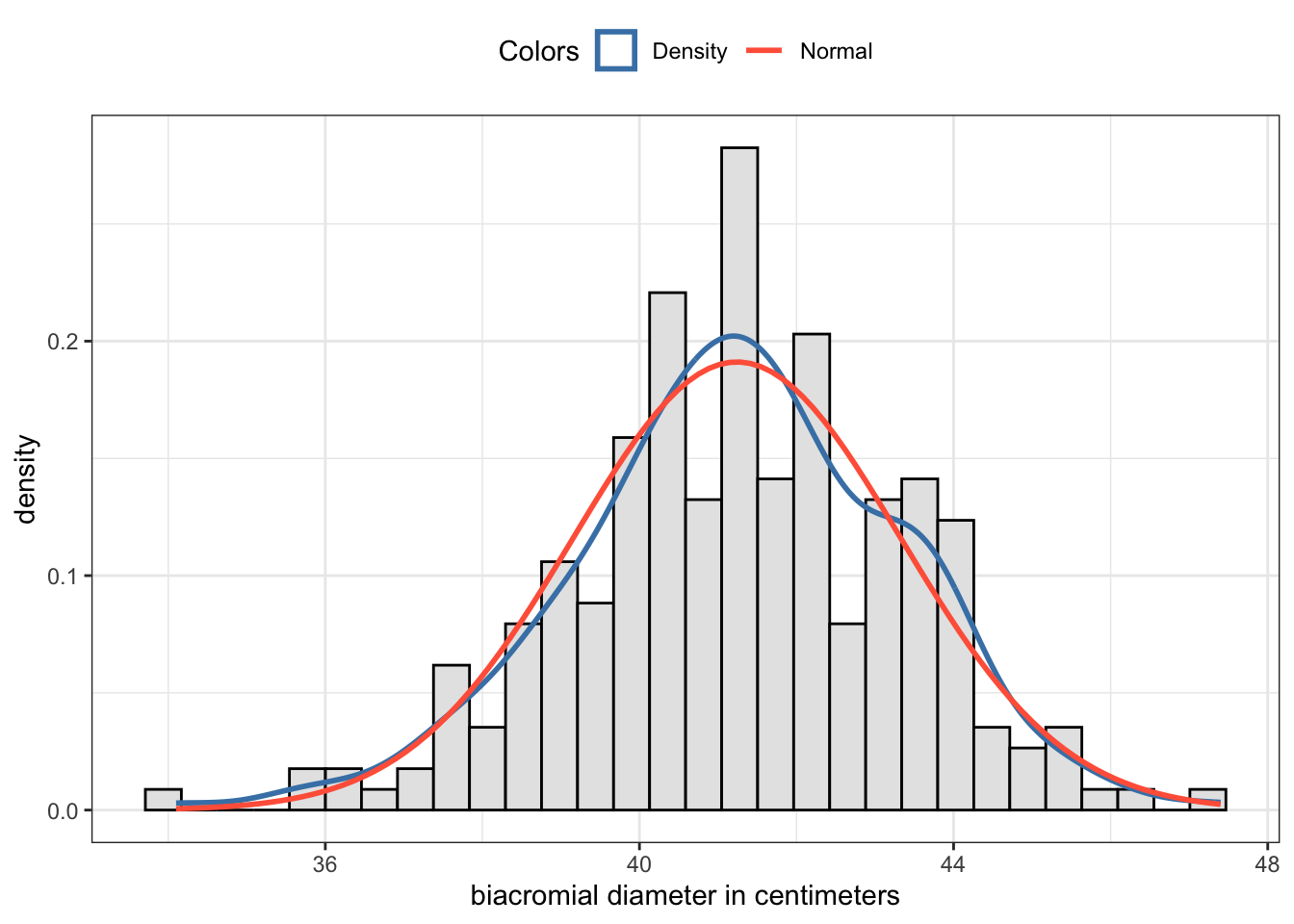
R Code 2.30 : Checking skewness of a shoulder breadth distribution of 247 men
Code
## select men from the samplebdims_male<-bdims|>dplyr::filter(sex==1)## construct graph using my private function my_hist_dnorm()p<-my_hist_dnorm(bdims_male, bdims_male$bia_di)p+ggplot2::labs(x ="biacromial diameter in centimeters")## commented test outputglue::glue("##################################################")glue::glue("Using the `semTools::skew()` function")semTools::skew(bdims_male$bia_di)glue::glue(" ")glue::glue("##################################################")glue::glue("Using the `statpsych::test.skew()` function")statpsych::test.skew(bdims$bia_di)
#> ##################################################
#> Using the `semTools::skew()` function
#>  skew (g1)         se          z          p
#> -0.2157434  0.1558573 -1.3842370  0.1662859
#>
#> ##################################################
#> Using the `statpsych::test.skew()` function
#>  Skewness      p
#>    0.1563 0.1464
(a) Shoulder breadth distribution in centimeters of 247 physically active men
Listing / Output 2.6: Checking skewness of a shoulder breadth distribution of 247 men
The interpretation follows Table 2.10: The \(z\) result of Graph 2.6 (a) from the biacromial diameter of 247 men is only 1.44, e.g. well situated in the range of -3.29 and +3.29 and therefore we have no skewness problem. The p-value is with 0.17 big and therefore the null (there is no skewness) can’t be rejected.
[statpsych::test.skew() c]omputes a Monte Carlo p-value (250,000 replications) for the null hypothesis that the sample data come from a normal distribution. If the p-value is small (e.g., less than .05) and the skewness estimate is positive, then the normality assumption can be rejected due to positive skewness. If the p-value is small (e.g., less than .05) and the skewness estimate is negative, then the normality assumption can be rejected due to negative skewness. (R Documentation of statpsych::test.skew())
Resource 2.3 Articles on identifying non-normal distributions
Harris referenced (Kim 2013) for the assessment table above. I noticed that there are many short articles about different types of test.. Just put the search string “Statistical[ALL] AND notes[ALL] AND clinical[ALL] AND researchers[ALL]” into the Kamje search engine.
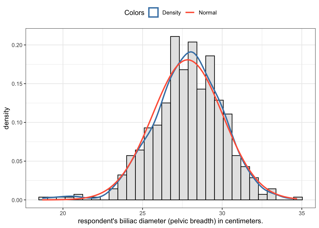
R Code 2.31 : Pelvic breadth distribution of 507 physically active individuals
Code
## construct graph using my private function my_hist_dnorm()p<-my_hist_dnorm(bdims, bdims$bii_di)p+ggplot2::labs(x ="respondent's biiliac diameter (pelvic breadth) in centimeters.")## commented test outputglue::glue("##################################################")glue::glue("Using the `semTools::skew()` function")semTools::skew(bdims$bii_di)glue::glue(" ")glue::glue("##################################################")glue::glue("Using the `statpsych::test.skew()` function")statpsych::test.skew(bdims$bii_di)
#> ##################################################
#> Using the `semTools::skew()` function
#>     skew (g1)            se             z             p
#> -0.4187365342  0.1087856586 -3.8491887572  0.0001185097
#>
#> ##################################################
#> Using the `statpsych::test.skew()` function
#>  Skewness     p
#>   -0.4175 1e-04
Graph 2.5: Pelvic breadth distribution in centimeters of 507 physically active indidviduals
Both tests have a very low p-value and attest us excessive skewness. This is even true if the z-value of semTools::skew() is only -3.85, e.g. in the appropriate boundaries of -7 and + 7 for a sample of 507 individuals (compare Table 2.10). The recommended visual inspection of the histogram shows us a left skewed distribution: There are too much individuals with a smaller pelvic breadth than it would appropriate for a normal distribution. It is very unlikely that the sample comes from a normal distribution. We have to reject the null.
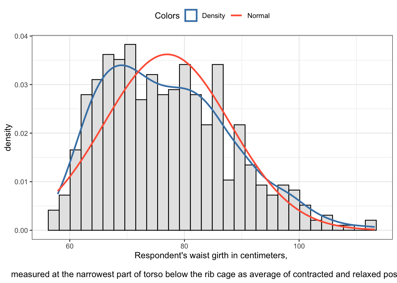
R Code 2.32 : Waist girth distribution in centimeters of 507 physically active individuals
Code
## construct graph using my private function my_hist_dnorm()p<-my_hist_dnorm(bdims, bdims$wai_gi)p+ggplot2::labs(x ="Respondent's waist girth in centimeters, \nmeasured at the narrowest part of torso below the rib cage as average of contracted and relaxed position")## commented test outputglue::glue("##################################################")glue::glue("Using the `semTools::skew()` function")semTools::skew(bdims$wai_gi)glue::glue(" ")glue::glue("##################################################")glue::glue("Using the `statpsych::test.skew()` function")statpsych::test.skew(bdims$wai_gi)
#> ##################################################
#> Using the `semTools::skew()` function
#>    skew (g1)           se            z            p
#> 5.422301e-01 1.087857e-01 4.984390e+00 6.215764e-07
#>
#> ##################################################
#> Using the `statpsych::test.skew()` function
#>  Skewness p
#>    0.5406 0
Graph 2.6: Waist girth distribution in centimeters of 507 physically active individuals
Both tests have a very low p-value and attest us excessive skewness. Again is the corresponding the z-value of semTools::skew() in the appropriate boundaries of -7 and + 7 for a sample of 507 individuals (compare Table 2.10). But the recommended visual inspection of the histogram shows us a right skewed distribution very clearly: There are too much individuals with a bigger waist girth than it would appropriate for a normal distribution. It is very unlikely that the sample comes from a normal distribution. We have to reject the null.
2.6.3 Mode
The book claims: “… unfortunately, perhaps because it is rarely used, there is no mode function.” This is not correct. There exists {modeest}, a package specialized for mode estimation (see Section A.49).
Harris therefore explains how to sort the variable to get the value most used as first item. This methods works always out of the box and does not need a specialized package.
R Code 2.33 : Most frequent value(s) in a given numerical vector
Code
tr_f<-forcats::fct_count(transgender_pb$TRNSGNDR)tr_recoded<-forcats::fct_count(transgender_clean$TRNSGNDR)|>dplyr::rename(Recoded ="f")tr<-dplyr::full_join(tr_f, tr_recoded, by =dplyr::join_by(n))|>dplyr::relocate(n, .after =dplyr::last_col())glue::glue("Let's remember the frequencies of the TRNSGNDR variable")trglue::glue(" ")glue::glue("#############################################")glue::glue("TRNSGDR variable not recoded and with NA's")transgender_pb|>dplyr::pull(TRNSGNDR)|>modeest::mfv()glue::glue(" ")glue::glue("#############################################")glue::glue("TRNSGDR variable not recoded with NA's")transgender_pb|>dplyr::pull(TRNSGNDR)|>modeest::mfv(na_rm =TRUE)glue::glue(" ")glue::glue("#############################################")glue::glue("TRNSGDR variable recoded without NA's")transgender_clean|>dplyr::pull(TRNSGNDR)|>modeest::mfv(na_rm =TRUE)
#> Let's remember the frequencies of the TRNSGNDR variable
#> # A tibble: 7 × 3
#>   f     Recoded                   n
#>   <fct> <fct>                 <int>
#> 1 1     Male to female          363
#> 2 2     Female to male          212
#> 3 3     Gender nonconforming    116
#> 4 4     Not transgender      150765
#> 5 7     Don’t know/Not sure    1138
#> 6 9     Refused                1468
#> 7 <NA>  <NA>                 310602
#>
#> #############################################
#> TRNSGDR variable not recoded and with NA's
#> [1] <NA>
#> Levels: 1 2 3 4 7 9
#>
#> #############################################
#> TRNSGDR variable not recoded with NA's
#> [1] 4
#> Levels: 1 2 3 4 7 9
#>
#> #############################################
#> TRNSGDR variable recoded without NA's
#> [1] Not transgender
#> 6 Levels: Male to female Female to male ... Refused
The function mfv() stands for Most Frequent Value(s) and is reexported by {modeest} from {statip}. It returns all modes, e.g. highest values from a vector. For instance: modeest::mfv(c("a", "a", "b", "c", "c")) returns “a, c”. If you want just the first mode value use modeest::mfv1().
R Code 2.34 Arrange data that most frequent value(s) are first row
Code
glue::glue("Let's remember the frequencies of the TRNSGNDR variable")trglue::glue(" ")glue::glue("#############################################. ")glue::glue("TRNSGDR variable with NA's")tr|>dplyr::arrange(desc(n))|>dplyr::dplyr_row_slice(1)glue::glue(" ")glue::glue("#############################################. ")glue::glue("TRNSGDR variable without NA's")tr|>tidyr::drop_na()|>dplyr::arrange(desc(n))|>dplyr::first()glue::glue(" ")glue::glue("#############################################. ")glue::glue("TRNSGDR variable without NA's: Just the mode value")tr|>tidyr::drop_na()|>dplyr::arrange(desc(n))|>dplyr::first()|>dplyr::pull(n)
#> Let's remember the frequencies of the TRNSGNDR variable
#> # A tibble: 7 × 3
#>   f     Recoded                   n
#>   <fct> <fct>                 <int>
#> 1 1     Male to female          363
#> 2 2     Female to male          212
#> 3 3     Gender nonconforming    116
#> 4 4     Not transgender      150765
#> 5 7     Don’t know/Not sure    1138
#> 6 9     Refused                1468
#> 7 <NA>  <NA>                 310602
#>
#> #############################################.
#> TRNSGDR variable with NA's
#> # A tibble: 1 × 3
#>   f     Recoded      n
#>   <fct> <fct>    <int>
#> 1 <NA>  <NA>    310602
#>
#> #############################################.
#> TRNSGDR variable without NA's
#> # A tibble: 1 × 3
#>   f     Recoded              n
#>   <fct> <fct>            <int>
#> 1 4     Not transgender 150765
#>
#> #############################################.
#> TRNSGDR variable without NA's: Just the mode value
#> [1] 150765
2.6.4 Kurtosis
2.6.4.1 What is kurtosis?
Kurtosis measures how many observations are in the tails of the distribution. If a distribution that looks bell-shaped has many observations in the tails it is more flat than a normal distribution and called platykurtic. On the other hand if a distribution has that looks bell-shaped has only a few observations in the tails it is more pointy than a normal distribution and called leptokurtic. A normal distribution is mesokurtic, e.g., it is neither platykurtic nor leptokurtic.
Platykurtic and leptokurtic deviations from normality do not necessarily influence the mean, since it will still be a good representation of the middle of the data if the distribution is symmetrical and not skewed. However, platykurtic and leptokurtic distributions will have smaller and larger values of variance and standard deviation, respectively, compared to a normal distribution. And this is a problem, as variance and standard deviation are not only used to quantify spread, but are also used in many of the common statistical tests.
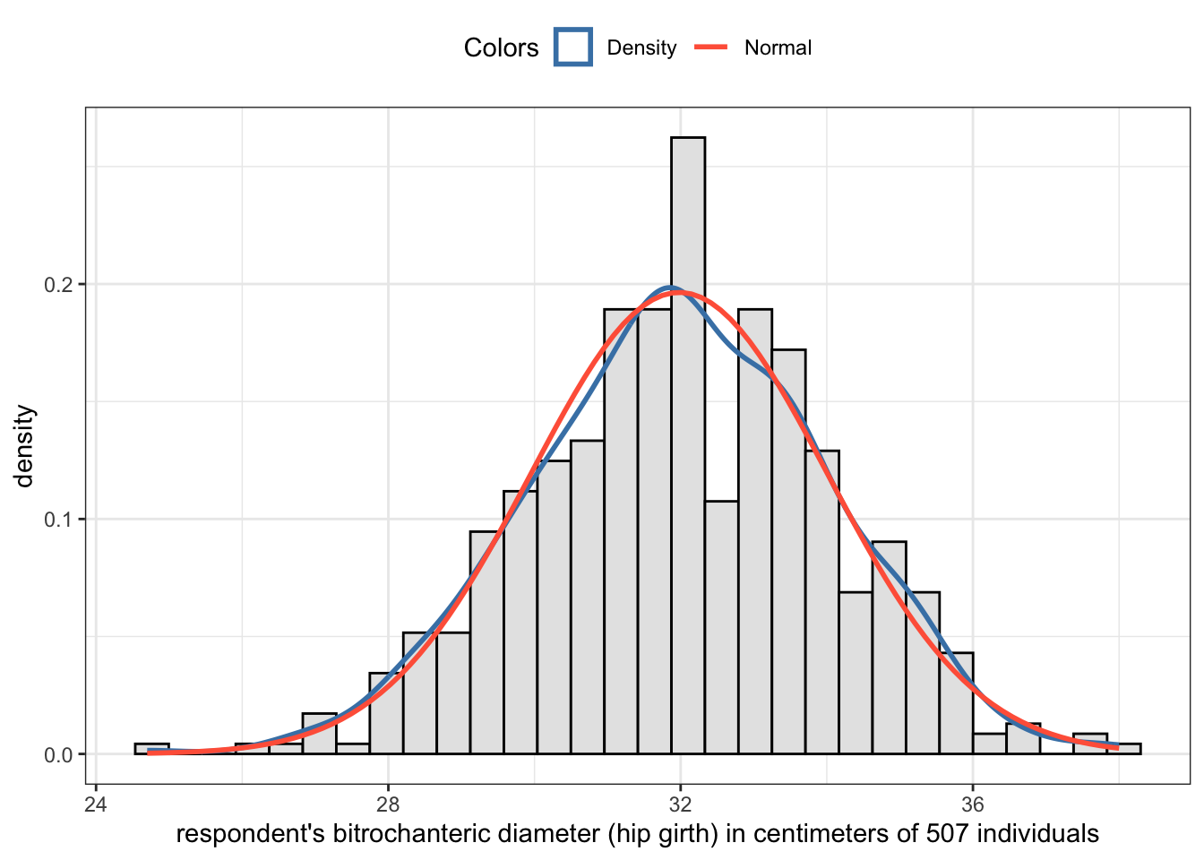
R Code 2.35 : Checking kurtosis of hip girth distribution of 507 individuals
Code
## construct graph using my private function my_hist_dnorm()p<-my_hist_dnorm(bdims, bdims$bit_di)p+ggplot2::labs(x ="respondent's bitrochanteric diameter (hip girth) in centimeters of 507 individuals")glue::glue("###################################################################")glue::glue("Kurtosis of pelvic breadth using `semTools::kurtosis()`")semTools::kurtosis(bdims$bit_di)glue::glue(" ")glue::glue("###################################################################")glue::glue("Kurtosis of pelvic breadth using `statpsych::test.kurtosis()`")statpsych::test.kurtosis(bdims$bit_di)
#> ###################################################################
#> Kurtosis of pelvic breadth using `semTools::kurtosis()`
#> Excess Kur (g2)              se               z               p
#>      0.04872448      0.21757132      0.22394715      0.82279843
#>
#> ###################################################################
#> Kurtosis of pelvic breadth using `statpsych::test.kurtosis()`
#>  Kurtosis Excess      p
#>    3.0364 0.0364 0.7486
Graph 2.7: Respondent’s bitrochanteric diameter (hip girth) in centimeters of 507 individuals
The excessive kurtosis computed by default is \(g_{2}\), the fourth standardized moment of the empirical distribution.
Kurtosis test of the pelvic breadth distribution
Both functions semTools::skew() and statpsych::test.skew() claim that there is no excess kurtosis. The z-value is small and the p-value is high, so we don’t have to reject the null: The probability is very high, that the data come from a normal distribution.
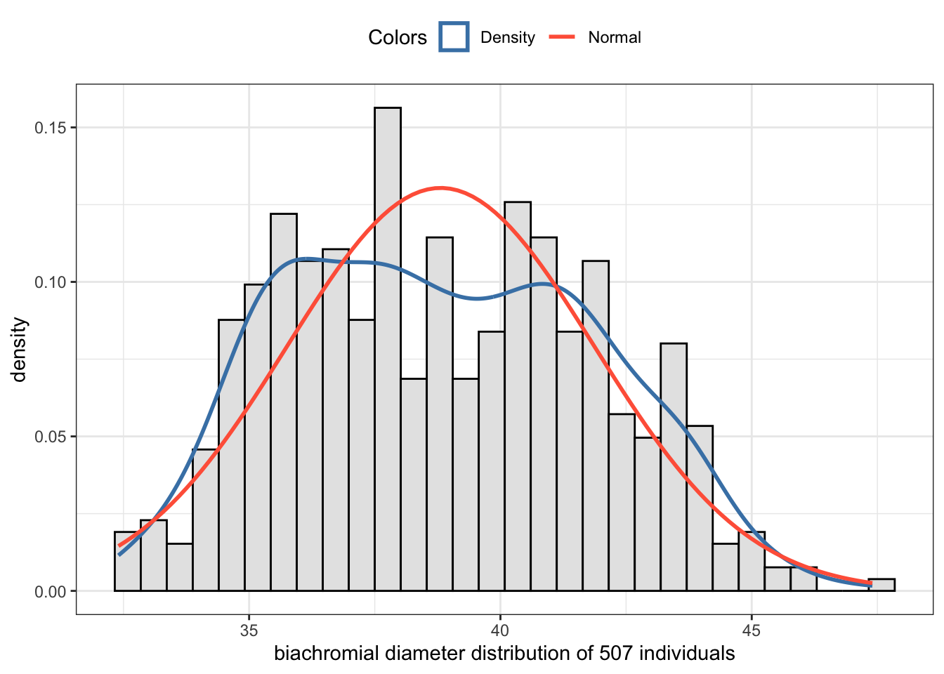
R Code 2.36 : Checking kurtosis of shoulder breadth distribution of 507 individuals
Code
## construct graph using my private function my_hist_dnorm()p<-my_hist_dnorm(bdims, bdims$bia_di)p+ggplot2::labs(x ="biachromial diameter distribution of 507 individuals")glue::glue("###################################################################")glue::glue("Kurtosis of biachromial diameter using `semTools::kurtosis()`")semTools::kurtosis(bdims$bia_di)glue::glue(" ")glue::glue("###################################################################")glue::glue("Kurtosis of biachromial diameter using `statpsych::test.kurtosis()`")statpsych::test.kurtosis(bdims$bia_di)
#> ###################################################################
#> Kurtosis of biachromial diameter using `semTools::kurtosis()`
#> Excess Kur (g2)              se               z               p
#>   -0.8258614973    0.2175713173   -3.7958197229    0.0001471564
#>
#> ###################################################################
#> Kurtosis of biachromial diameter using `statpsych::test.kurtosis()`
#>  Kurtosis  Excess p
#>    2.1704 -0.8296 0
Graph 2.8: Biachromial diameter (shoulder breadth) distribution of 507 individuals
Kurtosis test of the shoulder breadth distribution
Both functions semTools::skew() and statpsych::test.skew() assert that there is excess kurtosis. The p-value is very low, so we have to reject the null and assuming the alternative: The probability is very high, that the data didn’t come from a normal distribution.
As the z-value is below 3 and the excess value is negative we have a platykurtic (= flat) distribution. Looking at the histogram shows that this a reasonable interpretation.
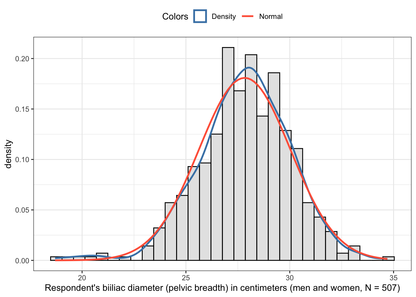
R Code 2.37 : Checking kurtosis of pelvis breadth distribution of 507 individuals
Code
## construct graph using my private function my_hist_dnorm()p<-my_hist_dnorm(bdims, bdims$bii_di)p+ggplot2::labs(x ="Respondent's biiliac diameter (pelvic breadth) in centimeters (men and women, N = 507)")glue::glue("###################################################################")glue::glue("Kurtosis of pelvis breadth distribution using `semTools::kurtosis()`")semTools::kurtosis(bdims$bii_di)glue::glue(" ")glue::glue("###################################################################")glue::glue("Kurtosis of pelvis breadth distribution using `statpsych::test.kurtosis()`")statpsych::test.kurtosis(bdims$bii_di)
#> ###################################################################
#> Kurtosis of pelvis breadth distribution using `semTools::kurtosis()`
#> Excess Kur (g2)              se               z               p
#>    1.112973e+00    2.175713e-01    5.115442e+00    3.130078e-07
#>
#> ###################################################################
#> Kurtosis of pelvis breadth distribution using `statpsych::test.kurtosis()`
#>  Kurtosis Excess     p
#>    4.0902 1.0902 5e-04
Graph 2.9: Respondent’s biiliac diameter (pelvic breadth) in centimeters of 507 individuals
Kurtosis test of the height distribution
Both functions semTools::skew() and statpsych::test.skew() assert that there is excess kurtosis. The p-value is very low, so we have to reject the null and assuming the alternative: The probability is very high, that the data didn’t come from a normal distribution.
As the z-value is above 3 and the excess value is positive we have a leptokurtic (= pointy) distribution. Looking at the histogram shows that this a reasonable interpretation.
Using only {semTools} for testing skewness and kurtosis
I haven’t found any difference between the results of {semTools} and {statpsych} in the computation of skewness and kurtosis. As the {statpsych} is more cumbersome, because of its 250,000 replications, I will stick with the {semTools} functions.
2.6.5 Scientifc notation
I have not troubles to read figures in scientific notation. But I often forget what command I must use to turn it off/on.
To turn off this option in R, type and run options(scipen = 999).
To turn it back on, type and run options(scipen = 000).
For graphs you could change the scale of the axis:
ggplot(aes(x = Year, y = num.guns/100000)) +
geom_line(aes(color = gun.type)) +
labs(y = "Number of firearms (in 100,000s)")
To turn off just for one variable: format(x, scientific = FALSE). It returns a character vector.
2.6.6 Data management for numerical variables
2.6.6.1 The book’s PHYSHLTH variable
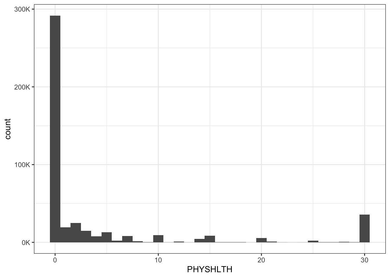
Example 2.4 : Data management for numerical PHYSHLTH variable
Concerning the first warning: bins = 30 wouldn’t be ideal, because we have 31 values (0-30 days where the physical health was not good). So bins = 31 would also be a good choice.
I have to confess that I didn’t know that one can use the argument na.rm = TRUE inside a {ggplot2} function.
2. Removing the scientific notation in the y-axis
At first I used used outside the {ggplot2}-block options(scipen = 999)`. But then I decided not to turn off generally the scientific notation but to find a solution inside of the {ggplot2} code chunk.
I came up with ggplot2::scale_y_continuous(labels = scales::label_number()). Using the {scales} package is a common way to change scales and labels of {ggplot2} graphics (see Section A.78). My command changed the scientific notation to numbers, but the numbers still had many zeros and are not handy.
Finally I found a general solution, without using the {scales} package: Writing a local function for the trans argument of the ggplot2::scale_y_continuous() directive. I didn’t know about this method before and found this solution on StackOverflow.
2.6.6.1.0.1 Central tendency
R Code 2.41 : Computing mean, median and mode of the PHYSHLTH variable
Code
physical_health_clean|>tidyr::drop_na()|>dplyr::summarize(mean =base::mean(PHYSHLTH), median =stats::median(PHYSHLTH), mode =modeest::mfv(PHYSHLTH))
#> # A tibble: 1 × 3
#>    mean median  mode
#>   <dbl>  <dbl> <dbl>
#> 1  4.22      0     0
2.6.6.1.0.2 Spread
R Code 2.42 : Computing standard deviation, variance, the IQR and the qunatiles of the PHYSHLTH variable
Code
physical_health_clean|>tidyr::drop_na()|>dplyr::summarize(sd =stats::sd(PHYSHLTH), var =stats::var(PHYSHLTH), IQR =stats::IQR(PHYSHLTH))glue::glue(" quantiles corresponding to the given probabilities")stats::quantile(physical_health_clean$PHYSHLTH, na.rm =TRUE)
#> # A tibble: 1 × 3
#>      sd   var   IQR
#>   <dbl> <dbl> <dbl>
#> 1  8.78  77.0     3
#>  quantiles corresponding to the given probabilities
#>   0%  25%  50%  75% 100%
#>    0    0    0    3   30
:::::
2.6.6.2 Achievement 3: The _AGE80 variable
Exercise 2.2 : Data management with the _AGE80 variable
#>      _AGE80
#>  Min.   :18.00
#>  1st Qu.:44.00
#>  Median :58.00
#>  Mean   :55.49
#>  3rd Qu.:69.00
#>  Max.   :80.00
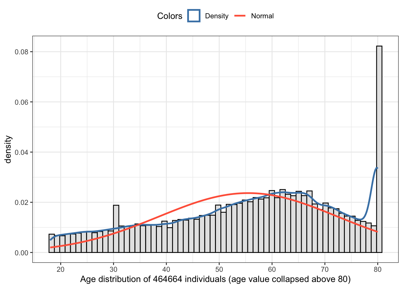
Graph 2.12: Imputed Age value collapsed above 80
Remember: I have used as column name _AGE80 (and not X_AGE80) when I imported with {haven} the data in Listing / Output 2.1.
The age of the respondents range from 18 to 80.
The good news: There are no missing values or other codes that we need to recode.
The bad news: The age value of 80 includes all people 80 and above. Therefore age 80 will have more observations as it would be appropriate for this age. As a consequence we can expect that the age distribution would be biased to the right (= left skewed). This is confirmed in two ways: (1) The median is higher than the mean and (2) we see the left skewed distribution also in the tiny histogram from the skimr::skim() summary.
R Code 2.44 : Central tendency, spread, skewness & kurtosis of _AGE80
Code
glue::glue("###################################################################")glue::glue("Central tendency and spread measures of `_AGE80` variable")age80|>dplyr::summarize( mean =base::mean(`_AGE80`), median =stats::median(`_AGE80`), mode =modeest::mfv(`_AGE80`), min =base::min(`_AGE80`), max =base::max(`_AGE80`), sd =stats::sd(`_AGE80`), var =stats::var(`_AGE80`), IQR =stats::IQR(`_AGE80`))## construct graph using my private function my_hist_dnorm()p<-my_hist_dnorm(age80, age80$`_AGE80`, n_bins =62)p+ggplot2::labs(x ="Age distribution of 464664 individuals (age value collapsed above 80)")+ggplot2::scale_x_continuous(breaks =seq(20,80,10))glue::glue(" ")glue::glue("###################################################################")glue::glue("Skewness of `_AGE80` variable")semTools::skew(age80$`_AGE80`)glue::glue(" ")glue::glue("###################################################################")glue::glue("Kurtosis of `_AGE80` variable")semTools::kurtosis(age80$`_AGE80`)
#> ###################################################################
#> Central tendency and spread measures of `_AGE80` variable
#> # A tibble: 1 × 8
#>    mean median  mode   min   max    sd   var   IQR
#>   <dbl>  <dbl> <dbl> <dbl> <dbl> <dbl> <dbl> <dbl>
#> 1  55.5     58    80    18    80  16.9  284.    25
#>
#> ###################################################################
#> Skewness of `_AGE80` variable
#>     skew (g1)            se             z             p
#> -4.002808e-01  3.593405e-03 -1.113932e+02  0.000000e+00
#>
#> ###################################################################
#> Kurtosis of `_AGE80` variable
#> Excess Kur (g2)              se               z               p
#>   -7.661943e-01    7.186809e-03   -1.066112e+02    0.000000e+00
Table 2.12: Age distribution of 464664 individuals (age value collapsed above 80)
As we already have assumed from the over sized 80 year value we have a left skewed distribution. But we have also excess kurtosis, because we have to much observation in the tails, e.g., the distribution is too flat (platykurtic) to come from a normal distribution.
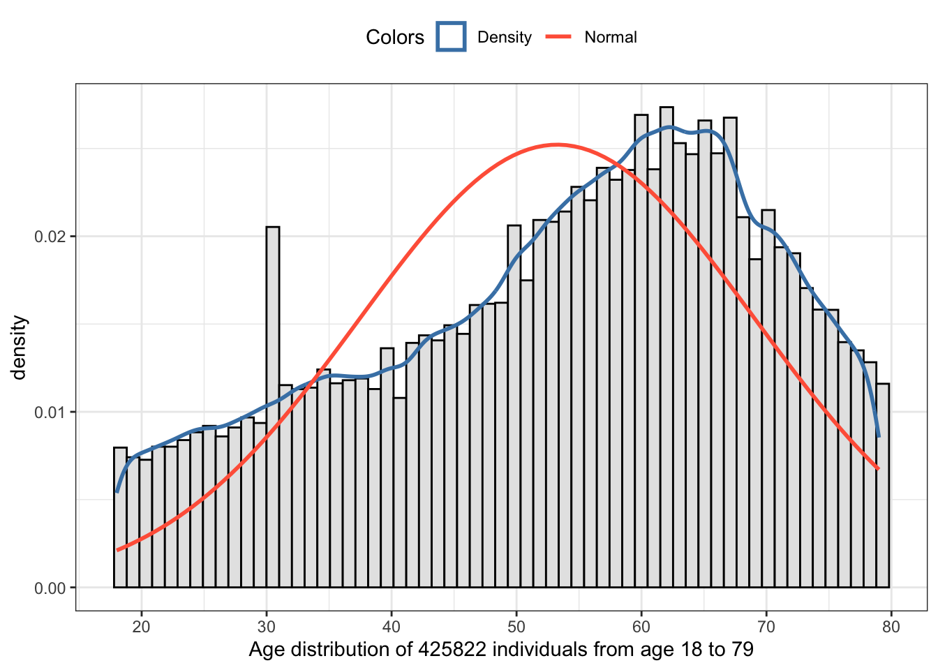
Now lets see the values after we have removed the obvious bias with the 80 year value. We will generate a new variable _AGE79 that range only from 18 to 79 years.
R Code 2.45 : Central tendency, spread, skewness & kurtosis of _AGE79
Code
glue::glue("###################################################################")glue::glue("Central tendency and spread measures of `_AGE79` variable")age79<-age80|>dplyr::filter(`_AGE80`<=79)|>dplyr::rename(`_AGE79` =`_AGE80`)age79|>dplyr::summarize( mean =base::mean(`_AGE79`), median =stats::median(`_AGE79`), mode =modeest::mfv(`_AGE79`), min =base::min(`_AGE79`), max =base::max(`_AGE79`), sd =stats::sd(`_AGE79`), var =stats::var(`_AGE79`), IQR =stats::IQR(`_AGE79`))## construct graph using my private function my_hist_dnorm()p<-my_hist_dnorm(age79, age79$`_AGE79`, n_bins =61)p+ggplot2::labs(x ="Age distribution of 425822 individuals from age 18 to 79")+ggplot2::scale_x_continuous(breaks =seq(20,80,10))glue::glue(" ")glue::glue("###################################################################")glue::glue("Skewness of `_AGE79` variable")semTools::skew(age79$`_AGE79`)glue::glue(" ")glue::glue("###################################################################")glue::glue("Kurtosis of `_AGE79` variable")semTools::kurtosis(age79$`_AGE79`)
#> ###################################################################
#> Central tendency and spread measures of `_AGE79` variable
#> # A tibble: 1 × 8
#>    mean median  mode   min   max    sd   var   IQR
#>   <dbl>  <dbl> <dbl> <dbl> <dbl> <dbl> <dbl> <dbl>
#> 1  53.3     56    62    18    79  15.8  250.    24
#>
#> ###################################################################
#> Skewness of `_AGE79` variable
#>     skew (g1)            se             z             p
#> -4.407561e-01  3.753717e-03 -1.174186e+02  0.000000e+00
#>
#> ###################################################################
#> Kurtosis of `_AGE79` variable
#> Excess Kur (g2)              se               z               p
#>   -7.528034e-01    7.507435e-03   -1.002744e+02    0.000000e+00
Table 2.13: Age distribution of 425822 individuals from age 18 to 79
Filtering the data to get only values between 18-79 doesn’t normalize the distribution. We can clearly see that there are too many people between 58 to 74 years respectively there is a gap in the cohorts from 35 to 55 years.
2.7 Creating tables for publishing
2.7.1 Necessary features
We need to manipulate data to provide a table with all its required features as they are:
Bullet List
A main title indicating what is in the table, including
the overall sample size
key pieces of information that describe the data such as the year of data collection and the data source
the units of measurement (people, organizations, etc.)
Correct formatting, including
consistent use of the same number of decimal places throughout the table
numbers aligned to the right so that the decimal points line up
words aligned to the left
indentation and shading to differentiate rows or sections
Clear column and row labels that have
logical row and column names
a clear indication of what the data are, such as means or frequencies
row and column sample sizes when they are different from overall sample sizes (Harris 2020).
I will use Table 2.5 (here it is Graph 2.13) from the book as my goal model that I want to replicate. In my first approach I will use {gtsummary} and document every step of the development process.
As first step I have reduced the dataset to those categories that are outlined in Graph 2.13. We will work with 222 records, 2 more as in the model table data are mentioned. But in the header it says “(n = 222)”.
R Code 2.47 Recode
Code
brfss_2014_recoded<-brfss_2014_raw|>dplyr::mutate(TRNSGNDR =forcats::as_factor(TRNSGNDR))|>dplyr::mutate(TRNSGNDR =forcats::fct_recode(TRNSGNDR, "Male to female"="1"))|>dplyr::mutate(TRNSGNDR =forcats::fct_recode(TRNSGNDR, "Female to male"="2"))|>dplyr::mutate(TRNSGNDR =forcats::fct_recode(TRNSGNDR, "Gender non-conforming"="3"))|>dplyr::mutate(`_AGEG5YR` =forcats::as_factor(`_AGEG5YR`))|>dplyr::mutate(`_AGEG5YR` =forcats::fct_recode(`_AGEG5YR`, "40-44"="5"))|>dplyr::mutate(`_AGEG5YR` =forcats::fct_recode(`_AGEG5YR`, "45-49"="6"))|>dplyr::mutate(`_AGEG5YR` =forcats::fct_recode(`_AGEG5YR`, "50-54"="7"))|>dplyr::mutate(`_AGEG5YR` =forcats::fct_recode(`_AGEG5YR`, "55-59"="8"))|>dplyr::mutate(`_AGEG5YR` =forcats::fct_recode(`_AGEG5YR`, "60-64"="9"))|>dplyr::mutate(`_AGEG5YR` =forcats::fct_recode(`_AGEG5YR`, "65-69"="10"))|>dplyr::mutate(`_AGEG5YR` =forcats::fct_recode(`_AGEG5YR`, "70-74"="11"))|>dplyr::mutate(`_RACE` =forcats::as_factor(`_RACE`))|>dplyr::mutate(`_RACE` =forcats::fct_recode(`_RACE`, "White"="1"))|>dplyr::mutate(`_RACE` =forcats::fct_recode(`_RACE`, "Black"="2"))|>dplyr::mutate(`_RACE` =forcats::fct_recode(`_RACE`, "Native American"="3"))|>dplyr::mutate(`_RACE` =forcats::fct_recode(`_RACE`, "Asian/Pacific Islander"="4"))|>dplyr::mutate(`_RACE` =forcats::fct_collapse(`_RACE`, "Other"=c("5", "7", "8", "9")))|>dplyr::mutate(`_INCOMG` =forcats::as_factor(`_INCOMG`))|>dplyr::mutate(`_INCOMG` =forcats::fct_recode(`_INCOMG`, "Less than $15,000"="1"))|>dplyr::mutate(`_INCOMG` =forcats::fct_recode(`_INCOMG`, "$15,000 to less than $25,000"="2"))|>dplyr::mutate(`_INCOMG` =forcats::fct_recode(`_INCOMG`, "$25,000 to less than $35,000"="3"))|>dplyr::mutate(`_INCOMG` =forcats::fct_recode(`_INCOMG`, "$35,000 to less than $50,000"="4"))|>dplyr::mutate(`_INCOMG` =forcats::fct_recode(`_INCOMG`, "$50,000 or more"="5"))|>dplyr::mutate(`_INCOMG` =forcats::fct_recode(`_INCOMG`, "Don't know/not sure/missing"="9"))|>dplyr::mutate(`_EDUCAG` =forcats::as_factor(`_EDUCAG`))|>dplyr::mutate(`_EDUCAG` =forcats::fct_recode(`_EDUCAG`, "Did not graduate highschool"="1"))|>dplyr::mutate(`_EDUCAG` =forcats::fct_recode(`_EDUCAG`, "Graduated highschool"="2"))|>dplyr::mutate(`_EDUCAG` =forcats::fct_recode(`_EDUCAG`, "Attended college/technical school"="3"))|>dplyr::mutate(`_EDUCAG` =forcats::fct_recode(`_EDUCAG`, "Graduated from college/technical school"="4"))|>dplyr::mutate(HLTHPLN1 =forcats::as_factor(HLTHPLN1))|>dplyr::mutate(HLTHPLN1 =forcats::fct_recode(HLTHPLN1, "Yes"="1"))|>dplyr::mutate(HLTHPLN1 =forcats::fct_recode(HLTHPLN1, "No"="2"))|>dplyr::mutate(PHYSHLTH =dplyr::case_match(PHYSHLTH, 77~NA,99~NA,88~0, .default =PHYSHLTH))|>labelled::set_variable_labels( TRNSGNDR ="Transition status", `_AGEG5YR` ="Age category", `_RACE` ="Race/ethnicity", `_INCOMG` ="Income category", `_EDUCAG` ="Education category", HLTHPLN1 ="Health insurance?", PHYSHLTH ="Days poor physical health per month")
WATCH OUT! Warning because of missing level 6 in _RACE variable
In my first run of this long R code I got the following warning:
My first try for a table 1 was just a one-liner with gtsummary::tbl_summary(). It looks already pretty good. But let’s compare with Graph 2.13 in detail:
My version is different in the header. It has “Characteristics” instead of “Survey participants demographics” and “N = 222” instead of “Frequency” and “Percentage” as separated columns.
My percentage values do not have one decimal place.
It is not obvious to which variable the “median, (IQR)” footnote belongs.
My labels are not bold.
I am not sure if I should account also for another difference: My “Health insurance” does not show the value “Yes” in a separate line. The same happens with “Days of poor physical health per month”. But I believe that my version is better as it prevents to show redundant information. My separate last line “Unknown” is in any case better, because it is an important information.
The first difference may be challenged for the same reason: Including “Frequency” and (braced) “Percentage” in one column and explained by a footnote is practically the same information just more compressed. It would provide more space for further information for more complex tables. So I will concentrate on number (2) to (4) and change in (1) only “Characteristic” to “Survey participants demographics”.
R Code 2.49 : Transgender Survey Participants Demographics (2nd try)
This would be the final result adapted to the features and possibilities of {gtsummary}. But just for the sake of learn more about {gtsummary} let’s separate frequencies and percent values into two columns. The advice in StackOverflow is to generate two table objects with the standard gtsummary::tbl_summary() and then to merge them with gtsummary::tbl:merge().
R Code 2.50 : Transgender Survey Participants Demographics (3rd try)
Code
tbl1_gtsummary<-brfss_2014_recoded|>gtsummary::tbl_summary( statistic =list(gtsummary::all_continuous()~"{median}",gtsummary::all_categorical()~"{n}"), label =PHYSHLTH~"Days poor physical health per month (median, IQR)")tbl2_gtsummary<-brfss_2014_recoded|>gtsummary::tbl_summary( statistic =list(gtsummary::all_continuous()~"({p25}, {p75})",gtsummary::all_categorical()~"{p}%"), digits =list(gtsummary::all_categorical()~1), label =PHYSHLTH~"Days poor physical health per month (median, IQR)")tbl_merge_gtsummary<-gtsummary::tbl_merge(list(tbl1_gtsummary, tbl2_gtsummary))|>gtsummary::bold_labels()|>gtsummary::modify_header(list(label~"**Survey participants demographics (N = {n})**",stat_0_1~"**Frequency**", stat_0_2~"**Percent**"))|>gtsummary::modify_spanning_header(gtsummary::everything()~NA)|>gtsummary::modify_footnote(gtsummary::everything()~NA)
#> Warning: The `update` argument of `modify_header()` is deprecated as of gtsummary 2.0.0.
#> ℹ Use `modify_header(...)` input instead. Dynamic dots allow for syntax like
#>   `modify_header(!!!list(...))`.
#> ℹ The deprecated feature was likely used in the gtsummary package.
#>   Please report the issue at <https://github.com/ddsjoberg/gtsummary/issues>.
The separation of the frequencies and percentages into two columns worked. But now we have an unfavorable line break in the first column with the variable labels. The problem is that the space between the columns are to wide, especially between second and third column.
I couldn’t find a way to reduce the space between columns. Maybe I would need to generate a new theme. But I have chosen to other possibilities:
The trick to get these details is to convert the {gtsummary} object with gtsummary::as_gt() into a {gt} object and then change the relevant characteristic. {gt} has much more control over the table display then {gtsummary} which has its strength to calculate and display values in a predefined table 1 style.
Here I have used the predefined compact theme with reduced font size and smaller cell paddings.
2.8 Exercises (empty)
I have skipped the chapter exercises: They bring nothing new for me. I have already done the recoding and table construction extensively and feel secure about these data management tasks.
2.9 Glossary
term
definition
Arithmetic Mean
The arithmetic mean, also known as "arithmetic average", is the sum of the values divided by the number of values. If the data set were based on a series of observations obtained by sampling from a statistical population, the arithmetic mean is the sample mean $\overline{x}$ (pronounced x-bar) to distinguish it from the mean, or expected value, of the underlying distribution, the population mean $\mu$ (pronounced /'mjuː/). (<a href="https://en.wikipedia.org/wiki/Mean">Wikipedia</a>)
Backtick
The backtick ` is a typographical mark used mainly in computing. It is also known as backquote, grave, or grave accent. (<a href="https://en.wikipedia.org/wiki/Backtick">Wikipedia</a>)
BRFSS
The Behavioral Risk Factor Surveillance System (BRFSS) is a system of health-related telephone surveys that collect state data about U.S. residents regarding their health-related risk behaviors, chronic health conditions, and use of preventive services. Established in 1984 with 15 states, BRFSS now collects data in all 50 states as well as the District of Columbia and three U.S. territories. BRFSS completes more than 400,000 adult interviews each year, making it the largest continuously conducted health survey system in the world. (<a href="https://www.cdc.gov/brfss/index.html">BRFSS</a>)
Cisgender
People whose gender identity matches their biological sex. Contrast: Transgender (SwR, Chapter 2)
CSV
Text files where the values are separated with commas (Comma Separated Values = CSV). These files have the file extension .csv
Data Tables
Data Tables are --- in contrast to Display Tables --- for analysis and not for presentation. Another purpose of Data Tables is to store, retrieve and share information digitally. In R they are tibbles, data.frames etc.
Deviation Scores
Deviation scores show the difference from some value like the mean; for example, z-scores show the deviation from the mean in standard deviation units
Display Tables
Display Tables are in constrast to Data Tables. You would find them in a web page, a journal article, or in a magazine. Such tables are for presentation, often to facilitate the construction of “Table 1”, i.e., baseline characteristics table commonly found in research papers. (<a href= "https://gt.rstudio.com/articles/gt.html">Introduction to Creating gt Tables</a>)
Frequencies
Frequencies are the number of times particular valuee of a variable occur. (SwR, Glossary)
Gender Nonconforming
Gender nonconforming means not adhering to society's gender norms. People may describe themselves as gender nonconforming if they don't conform to the gender expression, presentation, behaviors, roles, or expectations that society sees as the norm for their gender. ([APA Guidelines - PDF](https://www.apa.org/practice/guidelines/transgender.pdf))
Index of Qualitative Variation
The index of qualitative variation (IQV) is a type of statistic used to measure variation for nominal variables, which is often computed by examining how spread out observations are among the groups. (SwR, Glossary)
IQR
The interquartile range (IQR) is the upper and lower boundaries around the middle 50\% of the data in a numeric variable or the difference between the upper and lower boundaries around the middle 50\% of the data in a numeric variable. (SwR, Glossary)
Kurtosis
Kurtosis is a measure of how many observations are in the tails of a distribution; distributions that look bell-shaped, but have a lot of observations in the tails (platykurtic) or very few observations in the tails (leptokurtic) (SwR, Glossary)
Labelled Data
Labelled data (or labelled vectors) is a common data structure in other statistical environments to store meta-information about variables, like variable names, value labels or multiple defined missing values. (<a href="https://strengejacke.github.io/sjlabelled/articles/intro_sjlabelled.html">sjlabelled</a>)
Leptokurtic
Leptokurtic is a distribution of a numeric variable that has many values clustered around the middle of the distribution; leptokurtic distributions often appear tall and pointy compared to mesokurtic or platykurtic distributions. (SwR, Glossary)
MCMC
Markov chain Monte Carlo (MCMC) methods comprise a class of algorithms for sampling from a probability distribution. By constructing a [markov chain] that has the desired distribution as its equilibrium distribution, one can obtain a sample of the desired distribution by recording states from the chain. The more steps that are included, the more closely the distribution of the sample matches the actual desired distribution. Various algorithms exist for constructing chains. (<a href="https://en.wikipedia.org/wiki/Markov_chain_Monte_Carlo">Wikipedia</a>)
Median
Median is the middle value, or the mean of the two middle values, for a variable. (SwR, Glossary)
Mesokurtic
Mesokurtic are distributions that are neither platykurtic nor leptokurtic are mesokurtic; a normal distribution is a common example of a mesokurtic distribution. (SwR, Glossary)
Mode xy
Mode is the most common value of a variable. (SwR, Glossary)
p-value
The p-value is the probability that the test statistic is at least as big as it is under the null hypothesis (SwR, Glossary)
Percentages
Percentages are a relative values indicating hundredth parts of any quantity. (<a href="https://www.britannica.com/topic/percentage">Britannica</a>)
Platykurtic
Platykurtic is a distribution of a numeric variable that has more observations in the tails than a normal distribution would have; platykurtic distributions often look flatter than a normal distribution. (SwR, Glossary)
Quantile
Quantiles are cut points dividing the range of a probability distribution into continuous intervals with equal probabilities (<a href="https://en.wikipedia.org/wiki/Quantile">Wikipedia</a>)
Range
Range is the highest and lowest values of a variable, showing the full spread of values; the range can also be reported as a single number computed by taking the difference between the highest and lowest values of the variable. (SwR, Glossary)
Scientific Notation
Scientific notation is a way to display very large or very small numbers by multiplying the number by the value of 10 to some power to move the decimal to the left or right; for example, 1,430,000,000 could be displayed as 1.43 × 10^9 in scientific notation. (SwR, Glossary)
Skewness
Skewness is the extent to which a variable has extreme values in one of the two tails of its distribution (SwR, Glossary)
Standard Deviation
The standard deviation is a measure of the amount of variation or dispersion of a set of values. A low standard deviation indicates that the values tend to be close to the mean (also called the expected value) of the set, while a high standard deviation indicates that the values are spread out over a wider range. The standard deviation is the square root of its variance. A useful property of the standard deviation is that, unlike the variance, it is expressed in the same unit as the data. Standard deviation may be abbreviated SD, and is most commonly represented in mathematical texts and equations by the lower case Greek letter $\sigma$ (sigma), for the population standard deviation, or the Latin letter $s$ for the sample standard deviation. ([Wikipedia]
Standard Error
The standard error (SE) of a statistic is the standard deviation of its [sampling distribution]. If the statistic is the sample mean, it is called the standard error of the mean (SEM). (<a href="https://en.wikipedia.org/wiki/Standard_error">Wikipedia</a>) The standard error is a measure of variability that estimates how much variability there is in a population based on the variability in the sample and the size of the sample. (SwR, Glossary)
Table 1
Descriptive statistics are often displayed in the first table in a published article or report and are therefore often called <i>Table 1 statistics</i> or the <i>descriptives</i>. (SwR)
Transgender
Transgender people are people whose biological sex is not consistent with their gender. Contrast: [Cisgender] (SwR, Chapter 2)
Variance var
Variance is the squared deviation from the mean of a random variable. The variance is also often defined as the square of the standard deviation. Variance is a measure of dispersion, meaning it is a measure of how far a set of numbers is spread out from their average value. It is the second central moment of a distribution, and the covariance of the random variable with itself, and it is often represented by `σ`, `σ^2`, VAR(x), var(x) or V(x). ([Wikipedia](https://en.wikipedia.org/wiki/Variance))
Z-score
A z-score (also called a standard score) gives you an idea of how far from the mean a data point is. But more technically it’s a measure of how many standard deviations below or above the population mean a raw score is. (<a href="https://www.statisticshowto.com/probability-and-statistics/z-score/#Whatisazscore">StatisticsHowTo</a>)
Bonett, Douglas G. n.d. “Introduction to Categorical Data Analysis.”
Harris, Jenine K. 2020. Statistics With R: Solving Problems Using Real-World Data. Illustrated Edition. Los Angeles London New Delhi Singapore Washington DC Melbourne: SAGE Publications, Inc.
Heinz, Grete, Louis J. Peterson, Roger W. Johnson, and Carter J. Kerk. 2003. “Exploring Relationships in Body Dimensions.”Journal of Statistics Education 11 (2). https://doi.org/10.1080/10691898.2003.11910711.
Kim, Hae-Young. 2013. “Statistical Notes for Clinical Researchers: Assessing Normal Distribution (2) Using Skewness and Kurtosis.”Restorative Dentistry & Endodontics 38 (1): 52–54. https://doi.org/10.5395/rde.2013.38.1.52.
Narayan, Anand, Lizza Lebron-Zapata, and Elizabeth Morris. 2017. “Breast Cancer Screening in Transgender Patients: Findings from the 2014 BRFSS Survey.”Breast Cancer Research and Treatment 166 (3): 875–79. https://doi.org/10.1007/s10549-017-4461-8.
Wilcox, Allen R. 1973. “Indices of Qualitative Variation and Political Measurement.”The Western Political Quarterly 26 (2): 325–43. https://doi.org/10.2307/446831.
This was the original plan, but after several chapters working with the original data (downloading, recoding etc.) wasn’t instructive anymore. I didn’t learn new things because it was more a less a repetitive task with redundant code lines. So starting with Chapter 7 I have used the data files provided by the book and to strengthen my focus on the statistical issues.↩︎
Source Code
# Descriptive statistics {#sec-chap02}```{r}#| label: setup#| include: falsebase::source(file ="R/helper.R")```## Achievements to unlock::: {#obj-chap02}::: {.my-objectives}::: {.my-objectives-header}Objectives for chapter 02:::::: {.my-objectives-container}**SwR Achievements**- **Achievement 1**: (~~Understanding variable types and data types~~) (@sec-variable-data-types). As I already know this information I will skip this achievement. This empty section is only mentioned to get the same section numbering as in the book.- **Achievement 2**: Choosing and conducting descriptive analyses for categorical (factor) variables (@sec-chap02-describe-categorical-variables)- **Achievement 3**: Choosing and conducting descriptive analyses for continuous (numeric) variables (@sec-chap02-describe-numeric-variables)- **Achievement 4**: Developing clear tables for reporting descriptive statistics (@sec-chap02-create-tables-for-publishing)::::::Achievements for chapter 02:::## The transgender health care problemSubject of this chapter is the transgender health care problem.- `r glossary("Transgender")` people are people whose biological sex is not consistent with their gender.- `r glossary("Cisgender")` people are people whose gender identity matches their biological sex.In this chapter we are going to use data from the `r glossary("BRFSS")` website. The Behavioral Risk Factor Surveillance System (BRFSS) is a system of health-related telephone surveys that collect state data about U.S. residents regarding their health-related risk behaviors, chronic health conditions, and use of preventive services. Established in 1984 with 15 states, BRFSS now collects data in all 50 states as well as the District of Columbia and three U.S. territories. BRFSS completes more than 400,000 adult interviews each year, making it the largest continuously conducted health survey system in the world. (<a href="https://www.cdc.gov/brfss/index.html">BRFSS</a>)The rationale of this chapter is the fact, that prior to examiningstatistical relationships among variables, published studies in academicjournals usually present descriptive statistics. What kind of measures exist and how to describe the data set is an important task before one can start to analyse statistical relations. The followingscreenshot from [@narayan2017a, p.876] demonstrates how such descriptive statistics can be summarized to create a so-called`r glossary("Table 1")` as an introduction to the subject:[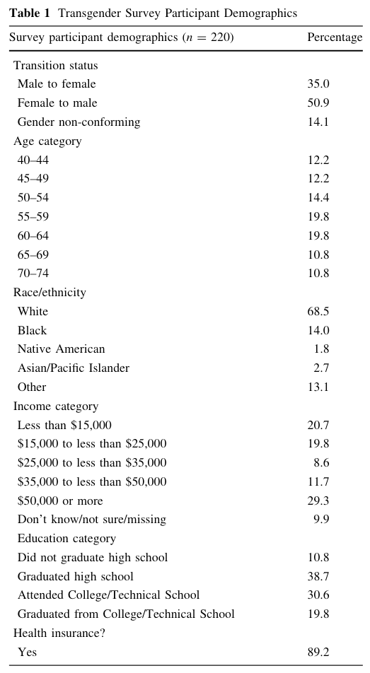{#fig-transgender-table1fig-alt="Screenshot of Table 1, \"Transgender Survey Participants Demographics\" from Narayan et. al. (2017)"}](https://link.springer.com/article/10.1007/s10549-017-4461-8)In this chapter we are going to reproduce @fig-transgender-table1 and add some additional information.## Data, codebook, and R packages::: {.my-resource}::: {.my-resource-header}:::::: {#lem-chap02-resources}: Data, codebook, and R packages for learning about descriptive statistics:::::::::::: {.my-resource-container}**Data**There are two options:1. Download the clean data file `transgender_hc_ch2.csv` from<https://edge.sagepub.com/harris1e>.2. Get the data file from the `r glossary("BRFSS")` website. (See @lst-chap02-get-brfss-2014-data). - The page with the 2014 data is at<https://www.cdc.gov/brfss/annual_data/annual_2014.html>. - The URL for the SAS transport file is at<http://www.cdc.gov/brfss/annual_data/2014/files/LLCP2014XPT.zip>.The ZIP-file is with 69 MB pretty big. Unzipped it will have almost 1GB! --- I will only work with this second option[^chap02-1].[^chap02-1]: This was the original plan, but after several chapters working with the original data (downloading, recoding etc.) wasn't instructive anymore. I didn't learn new things because it was more a less a repetitive task with redundant code lines. So starting with @sec-chap07 I have used the data files provided by the book and to strengthen my focus on the statistical issues.**Codebook**Again there are two options:1. Download `brfss_2014_codebook.pdf` from<https://edge.sagepub.com/harris1e>.2. Download the codebook as PDF from the BRFSS webpage. - The location of the codebook is the same as above:<https://www.cdc.gov/brfss/annual_data/annual_2014.html>. - The PDF codebook (2.74 MB) can be found at[https://www.cdc.gov/brfss/annual_data/2014/pdf/CODEBOOK14_LLCP.pdf](https://www.cdc.gov/brfss/annual_data/annual_2014.html)**Packages**1. Packages used with the book (sorted alphabetically): - descr (@sec-descr) - haven (@sec-haven) - kableExtra {@sec-kableExtra} - knitr - tidyverse (@sec-tidyverse) - dplyr (@sec-dplyr) - ggplot2 (@sec-ggplot2) - forcats (@sec-forcats) - tidyr (@sec-tidyr) - tableone - semTools (@sec-semTools) - qualvar (@sec-qualvar) - labelled (@sec-labelled) - Hmisc (@sec-Hmisc)2. My additional packages (sorted alphabetically) - gtsummary (@sec-gtsummary) - skimr (@sec-skimr)::::::## Understanding variable types and data types {#sec-variable-data-types}### IntroductionTo know about variable and data types is essential as different typesrequire different approaches for the analysis. The following outline of the next sections is slightly adapted from the book. Harris has some measures of categorical variables (mode and index of qualitative variation) explained in the section on numeric variables.- **Categorical variables**: - **Central tendency**: The two most commonly used and reported descriptive statistics for categorical (or factor) data types are `r glossary("frequencies")` and `r glossary("percentages")`. Sometimes also the `r glossary("mode xy", "mode")` is used to identify the most common (or typical) category of a factor variable. - **Spread / Variety**: is for for categorical variables not often reported. Harris mentions the `r glossary("index of qualitative variation")`, which quantifies how much the observations are spread across the categories of a categorical variable.- **Numerical variables**: - **Central tendency**: The most important measures are the `r glossary("arithmetic mean", "mean")`, `r glossary("median")` and `r glossary("mode xy", "mode")`. - **Spread**: - in relation to the mean: the `r glossary("variance var", "variance")` and `r glossary("standard deviation")` - in relation to the median: `r glossary("range")`, `r glossary("IQR", "interquartile range")` (IQR) and `r glossary("quantile")`.For the decision if one should report mean or median in numerical variables the measures for `r glossary("skewness")` and `r glossary("kurtosis")` are helpful. Another issue with numerical variables is usage of `r glossary("scientific notation")`.I will explain explicitly only to those subjects where I am not firm. This is ::: {#bul-subjects-explained}:::::{.my-bullet-list}:::{.my-bullet-list-header}Bullet List:::::::{.my-bullet-list-container}- categorical variables: - index of qualitative variation (@sec-index-variation)- numeric variables: - skewness (@sec-chap02-skewness) - mode (@sec-chap02-mode) - kurtosis (@sec-chap02-kurtosis) - scientific notation:::::::::Subjects reviewed in this chapter:::***But I will address all the other measures in the examples resp. exercises.### Get the dataBut before we are going to work with the data we have do download it form the `r glossary("BRFSS")` website. ::: {.callout-warning}Downloading the huge file (69 MB as ZIP and 1 GB unzipped) will takesome minutes. So be patient!::::::::{.my-r-code}:::{.my-r-code-header}:::::: {#cnj-chap02-get-brfss-2014-data}: Download the SAS transport file data from the BRFSS website and savedataframe with selected variables as R object:::::::::::::{.my-r-code-container}:::{#lst-chap02-get-brfss-2014-data}```{r}#| label: get-brfss-2014-data#| eval: false#| cache: true## run this code chunk only once (manually)url <-"http://www.cdc.gov/brfss/annual_data/2014/files/LLCP2014XPT.zip"utils::download.file(url = url,destfile = tf <- base::tempfile(),mode ="wb")brfss_2014 <- haven::read_xpt(tf)brfss_tg_2014 <- brfss_2014 |> dplyr::select( TRNSGNDR, `_AGEG5YR`, `_RACE`, `_INCOMG`, `_EDUCAG`, HLTHPLN1, HADMAM, `_AGE80`, PHYSHLTH)data_folder <- base::paste0(here::here(), "/data/")if (!base::file.exists(data_folder)) {base::dir.create(data_folder)}chap02_folder <- base::paste0(here::here(), "/data/chap02/")if (!base::file.exists(chap02_folder)) {base::dir.create(chap02_folder)}base::saveRDS(object = brfss_tg_2014, file =paste0(chap02_folder, "/brfss_tg_2014_raw.rds"))```Download and save the transgender data 2014 from the BRFSS website:::***The original file has 279 variables and 464664 observations. After selectingonly 9 variable the file is with 31.9 MB (memory usage) and storedcompressed (2.2 MB) much smaller.::: my-note::: my-note-headerFour observations about the code:::::: my-note-container1. It is not possible to download the file with`haven::read_xpt(<URL>)` directly. At first one has to create a temporary file to store the zipped file.2. Whenever you meet a variable / row name with a forbidden R syntax surround the name with `r glossary("backtick", "backticks")` ([grave accents](https://en.wikipedia.org/wiki/Grave_accent)).3. Instead of exporting the R object into a `r glossary("CSV", ".csv")` file I save the data as a compressed R object that can loaded easily again into the computer memory with the `base::readRDS()` function.4. With regard to the `base::saveRDS()` function I have to remind myself that the first argument is the R object *without* quotes. I committed this error several times.:::::::::::::::## Descriptive analyses for categorical (factor) variables {#sec-chap02-describe-categorical-variables}The goal of this section is to summarize and interpret the categorical variable `TRNSGNDR`. In contrast to the book I will work with a dataframe consisting only of the variable which I will recode to `transgender`.### Summarize categorical variables without recoding::: my-example::: my-example-header::: {#exm-chap02-interpret-categorical-variables}: Summarize categorical variables without recoding::::::::: my-example-container::: panel-tabset###### select()```{r}#| label: select-transgenderchap02_folder <- base::paste0(here::here(), "/data/chap02/")## create transgender_pb ########## as intermediate datatransgender_pb <- base::readRDS(base::paste0(chap02_folder, "brfss_tg_2014_raw.rds")) |> dplyr::select(TRNSGNDR)base::saveRDS(object = transgender_pb, file = base::paste0(chap02_folder, "transgender_pb.rds"))```(*This code chunk has no visible output.*)###### str()::: my-r-code::: my-r-code-header::: {#cnj-chap02-str-transgender}: Show structure of the `transgender` data with `utils::str()`::::::::: my-r-code-container```{r}#| label: str-transgender#| lst-label: lst-chap02-str-transgender#| lst-cap: "Show structure of the `transgender` data with `utils::str()`"#| cache: trueutils::str(transgender_pb)```***{**haven**} has imported `r glossary("labelled data")` for the variables. We can use these labels to find the appropriate passages in the 126 pages of thecodebook. Just copy the variable label and search this string inthe PDF of the codebook.------------------------------------------------------------------------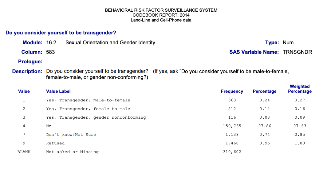{#fig-chap02-codebook-transgenderfig-alt="The table displays the sexual orientation and gender identity as an answer of the question 'Do you consider yourself to be transgender?' - The answers were: Yes, male-to-female: 363; Yes, female-to-male: 212; Yes, gender nonconforming: 116; No: 150,765; Don't know / Not sure: 1,138; Refused: 1,468; Not asked or missing: 310,602."}::::::Note that variable labels are restricted to 40 characters. I thinkthis is an import limitation of {**haven**} because there is no suchrestriction using `haven::labelled()`. But we need to recode the dataanyway, especially as there are no value labels available.###### summary()::: my-r-code::: my-r-code-header::: {#cnj-chap02-summary-transgender}: Summarize `transgender` data with `base::summary()`::::::::: my-r-code-container```{r}#| label: summary-transgender#| cache: truebase::summary(transgender_pb)```***If categories have no labels for their levels, then the `summary()` function is useless.::::::###### skim()::: my-r-code::: my-r-code-header::: {#cnj-chap02-skim-transgender}: Summarize transgender data with `skimr::skim()`::::::::: my-r-code-container```{r}#| label: skim-transgender_pb#| cache: trueskimr::skim(transgender_pb)```Again: As long as the categorical variable is of numeric class all the statistics about the distribution of the level values are pointless.::::::###### gtsummary()::: my-r-code::: my-r-code-header::: {#cnj-chap02-gtsummary-transgender}: Summarize and display transgender data with `gtsummary::tbl_summary()`::::::::: my-r-code-container```{r}#| label: tbl-gtsummary-transgender#| tbl-cap: "A firt approach to produce a 'Table 1' statistics with {gtsummary} using labelled data"#| cache: truegtsummary::tbl_summary(transgender_pb)```------------------------------------------------------------------------{**gtsummary**} uses here the labelled data imported with {**haven**}.Not bad, isn't it? Just a one-liner produces this first trial for a pbulic ready`r glossary("Table 1")` statistics. This first attempt of table would beeven better if the data had also value labels. For moreinformation how to work with with labelled data see the full@sec-chap01-labelled-data with all its sub-sections. You will findsome functions how to adapt @tbl-gtsummary-transgender to get a betterdescriptive in @sec-chap01-experiments-gtsummary. But follow also this chapteralong!:::::::::::::::To summarize a categorical variable without recoding is generally not purposeful. An exception is `utils::str()` as it display the internal structure including attributes. With `utils::str()` one can detect for example if the data are labelled. If this is the case a quick glance at the data with `gtsummary::tbl_summary()` could be sensible.### Convert numerical variable to factor and recode its levels:::::{.my-procedure}:::{.my-procedure-header}Categorical variable: Four steps to get sensible values for reporting data:::::::{.my-procedure-container}1. To print a basic `table()` is always a useful first try.2. Check the `class()` of the variable. For a categorical variable is has to be `factor`.3. If this not the case then you have to recode the variable `forcats::as_factor`.4. Then you can `forcats::fct_count()` the different levels of the factor.5. Finally you can now recode the levels of the factor variable with `forcats::fct_recode()` to match the description in the codebook.:::::::::::: my-example::: my-example-header::: {#exm-chap02-data-wrnagling-categorical}: Convert numerical variable to factor and recode its level::::::::: my-example-container::: panel-tabset###### table()::: my-r-code::: my-r-code-header::: {#cnj-code-chap02-table-transgender}: Using `base::table()` to count factor levels::::::::: my-r-code-container```{r}#| label: table-transgender## load transgender_pb ##########chap02_folder <- base::paste0(here::here(), "/data/chap02/")transgender_pb <- base::readRDS(base::paste0(chap02_folder, "transgender_pb.rds"))base::table(transgender_pb$TRNSGNDR)```------------------------------------------------------------------------Compare the values with the screenshot from the codebook in@fig-chap02-codebook-transgender.::::::Normally `table()` is used for cross-classifying factors to build a contingency table of the counts at each combination of factor levels. But here I have only one variable.###### class():::::{.my-r-code}:::{.my-r-code-header}:::::: {#cnj-chap02-class-transgender}: Check class of categorical variable `TRNSGNDR```:::::::::::::{.my-r-code-container}```{r}#| label: class-transgenderclass(transgender_pb$TRNSGNDR)```:::::::::###### as_factor():::::{.my-r-code}:::{.my-r-code-header}:::::: {#cnj-chap02-as-factor-transgender}: Convert numerical variable TRNSGNDR to categorical variable:::::::::::::{.my-r-code-container}```{r}#| label: as-factor-transgendertransgender_pb$TRNSGNDR <- forcats::as_factor(transgender_pb$TRNSGNDR)class(transgender_pb$TRNSGNDR)```Instead of `base::as.factor()` I am using `as_factor()` from the {**forcats**} package which is part of the {**tidyverse**} collection. See @sec-forcats.:::::::::###### fct_count():::::{.my-r-code}:::{.my-r-code-header}:::::: {#cnj-get-levels}: Get information about the levels of a factor variable:::::::::::::{.my-r-code-container}```{r}#| label: get-levelstransgender_pb |> dplyr::pull(TRNSGNDR) |> forcats::fct_count()```***`forcats::fct-count()` gives you all the information you need to recode a categorical variable:1. You will see the number of `NA`s.2. And even more important: If there are (currently) unused levels then `forcats::fct_count()` will also list them as $0$ observations.3. You will see if some levels are not used much so you can decide if you should probably merge them to a category of "other". {**forcats**} has several function to support you in this task.:::::::::You can now recode the levels according to the information in the codebook (see @fig-chap02-codebook-transgender).###### fct_recode()::: my-r-code::: my-r-code-header::: {#cnj-chap02-recode-transgender}: Recode the `TRNSGNDR` variable to match the codebook levels::::::::: my-r-code-container::: {#lst-chap02-recode-transgender}```{r}#| label: recode-transgender#| results: hold## create transgender_clean #########transgender_clean <- transgender_pb |> dplyr::mutate(TRNSGNDR = forcats::fct_recode(TRNSGNDR,"Male to female"='1',"Female to male"='2',"Gender nonconforming"='3',"Not transgender"='4',"Don’t know/Not sure"='7',"Refused"='9' )) base::summary(transgender_clean)## saving the variable is useful in the developing stage## it helps to work with individual code chunks separatelychap02_folder <- base::paste0(here::here(), "/data/chap02/")base::saveRDS(object = transgender_clean, file = base::paste0(chap02_folder, "transgender_clean.rds"))```Recoded `TRNSGNDR` variable to match the codebook levels:::::::::Harris explains in the book the superseded function `dplyr::recode_factor()`. It's new equivalent is now `forcats::fct_recode()`.:::::::::### Data management#### Display categorical variable for reports After recoding `TRNSGNDR` we have in @lst-chap02-recode-transgender printed the resulted tibble. The output summarizes already understandable the essence of the variable. But we are still missing some information:1. Besides the frequencies we need also the percentages to better understand the data.2. As there is a huge amount of missing data, we need to calculate these percentages with and without NA's.In the following example we discuss functions of different packages to get the desired result.::: my-example::: my-example-header::: {#exm-chap02-data-wrangling-categorical}: Data management to display categorical variable for reports ::::::::: my-example-container::: panel-tabset###### skim():::::{.my-r-code}:::{.my-r-code-header}:::::: {#cnj-chap02-skim-transgender-clean}: Display summary of the `TRNSGNDR` variable with `skimr::skim()`:::::::::::::{.my-r-code-container}```{r}#| label: skim-transgender-cleanskimr::skim(transgender_clean)```***The result of `skimr::skim()` for categorical variable is somewhat disappointing. It does not report the levels of the variable. The abbreviations of the top counts (4 levels of 6) are not understandable.:::::::::###### describe():::::{.my-r-code}:::{.my-r-code-header}:::::: {#cnj-chap02-describe-transgender}: Display summary of the `TRNSGNDR` variable with `Hmisc::describe()`:::::::::::::{.my-r-code-container}```{r}#| label: describe-transgender## load transgender_clean ##########chap02_folder <- base::paste0(here::here(), "/data/chap02/")transgender_clean <- base::readRDS(base::paste0(chap02_folder, "transgender_clean.rds"))Hmisc::describe(transgender_clean)```***`Hmisc::describe()` is a completely new function for me. Sometimes I met in my reading the {**Hmisc**} package, but I have never applied functions independently. (Fore more information on {**Hmisc**} see @sec-Hmisc.)In contrast to other methods it does not list the levels vertically but horizontally. This is unfortunately not super readable and one needs --- at least in this case --- to use the horizontal scroll bar.But is has the advantage to display not only the frequencies but also the percentages.:::::::::###### {report}:::::{.my-r-code}:::{.my-r-code-header}:::::: {#cnj-chap02-report-transgender}: Display summary of the `TRNSGNDR` variable with `report::report_table()`:::::::::::::{.my-r-code-container}```{r}#| label: report-transgender#| comment: ''#| results: markupreport::report_table(transgender_clean)```I just learned about the existence of {**report**}. It is specialized to facilitate reporting of results and statistical models (See: @sec-report). The one-liner shows the levels of the variable, frequencies (`n_obs`) and percentages. Not bad!In this example I have used the `report::report_table()` function because the verbal result of the standard `report::report()` function is rather underwhelming as you can see: ***`r report::report(transgender_clean)`***Compare this to the example of the book:::: {#rep-chap02-transgender1}::: {.callout-tip style="color: darkgreen;"}The 2014 BRFSS had a total of 464,664 participants. Of these, 310,602 (66.8%) were not asked or were otherwise missing a response to the `r glossary("transgender")` status question. A few participants refused to answer (n = 1,468; 0.32%), and a small number were unsure of their status (n = 1,138; 0.24%). Most reported being not transgender (n = 150,765; 32.4%), 116 were `r glossary("gender nonconforming", "gender non-conforming")` (0.03%), 212 were female to male (0.05%), and 363 were male to female (0.08%).:::Do you consider yourself to be transgender? (Figures with missing values):::(There is another report of the `TRNSGNDR` without the many `NA`s: See @rep-chap02-transgender2 for a comparison.)But it seems to me that with more complex results (e.g., reports from models) {**report**} is quite useful. In the course of this book I will try it out and compare with the reports of other functions.***Another thought: I have filed an issue because I think that it would be a great idea to provide a markdown compatible table so that Quarto resp. pandoc could interpret as a table and visualizing it accordingly. The table above would then appear as the following (copied and slightly edited) example:Variable | Level | n_Obs | percentage_Obs---------|----------------------|--------|----------------TRNSGNDR | Male to female | 363 | 0.08TRNSGNDR | Female to male | 212 | 0.05TRNSGNDR | Gender nonconforming | 116 | 0.02TRNSGNDR | Not transgender | 150765 | 32.45TRNSGNDR | Don’t know/Not sure | 1138 | 0.24TRNSGNDR | Refused | 1468 | 0.32TRNSGNDR | missing | 310602 | 66.84: Slightly modified {**report**} table to get a Markdown compatible table:::::::::###### na.omit():::::{.my-r-code}:::{.my-r-code-header}:::::: {#cnj-chap02-na-omit-transgender}: Display summary of the `TRNSGNDR` variable with the recoding method from the book:::::::::::::{.my-r-code-container}```{r}#| label: na-omit-transgendertransgender_clean |> dplyr::group_by(TRNSGNDR) |> dplyr::summarize(n = dplyr::n()) |> dplyr::mutate(perc_all =100* (n /sum(n))) |> dplyr::mutate(perc_valid =100* (n /sum(n[na.omit(TRNSGNDR)])))```::::::::::::::{.my-watch-out}:::{.my-watch-out-header}WATCH OUT! Wrong `perc_valid` cell value in `NA` row:::::::{.my-watch-out-container}I have the same logic used as the author in the book and got the same result too. But the result of one cell is wrong! The `perc_valid` cell value in the `NA` row should be empty, but it shows the value 202 (rounded).:::::::::###### freq():::::{.my-r-code}:::{.my-r-code-header}:::::: {#cnj-chap02-freq-transgender}: Display summary of the `TRNSGNDR` variable with `descr::freq()`:::::::::::::{.my-r-code-container}::: {#lst-chap02-freq-transgender}```{r}#| label: freq-transgenderdescr::freq(transgender_clean$TRNSGNDR, plot =FALSE)```Using `descr::freq()` to calculate values with and without NA's:::This is the first time I used the {**descr**} package and it shows so far the best result! (See @sec-descr.) The one-liner shows levels, frequencies, percentage with and without missing values. It even plots a bar graph, but this is not useful here, so I omitted it with `plot = FALSE`.The only disadvantage: One has to learn a new package. And --- searching about packages about descriptive statistics I learned that there are at least 10 other packages. :::::::::###### {tidyverse}:::::{.my-r-code}:::{.my-r-code-header}:::::: {#cnj-chap02-full-join-transgender}: Display summary of the `TRNSGNDR` variable with my recoding method using {**dplyr**} and {**tidyr**} from the {**tidyverse**}:::::::::::::{.my-r-code-container}```{r}#| label: full-join-transgendertg1 <- transgender_clean |> dplyr::group_by(TRNSGNDR) |> dplyr::summarize(n = dplyr::n()) |> dplyr::mutate(perc_all =100* (n /sum(n)))tg2 <- transgender_clean |> dplyr::group_by(TRNSGNDR) |> tidyr::drop_na() |> dplyr::summarize(n = dplyr::n()) |> dplyr::mutate(perc_valid =100* (n /sum(n)))dplyr::full_join(tg1, tg2, by = dplyr::join_by(TRNSGNDR, n))```Here I created a tibble with frequencies and percentages with and another one without missing data. Then I join these two tibbles together.Although this code with packages from the {**tidyverse**} collection is more complex and verbose than the one-liner from @lst-chap02-freq-transgender using {**descr**} it has the advantage that one does not need to install and learn a new package. I believe that sometimes it is more efficient to be proficient with some packages than to know many packages superficially.:::::::::::: {#rep-chap02-transgender2}::: {.callout-tip style="color: darkgreen;"}The 2014 BRFSS had a total of 464,664 participants. Of these, 310,602 (66.8%) were not asked or were otherwise missing a response to the `r glossary("transgender")` status question. Of the 33.2% who responded, some refused to answer (n = 1,468; 0.95%), and a small number were unsure of their status (n = 1,138, 0.74%). Most reported being not transgender (n = 150,765; 97.9%), 116 were `r glossary("gender nonconforming", "gender non-conforming")` (0.08%), 212 were female to male (0.14%), and 363 were male to female (0.24%).:::Do you consider yourself to be transgender? (Figures without missing values):::Compare with @rep-chap02-transgender1.:::::::::#### Index of qualitative variation {#sec-index-variation}##### IntroductionThe `r glossary("index of qualitative variation")` (IQV) quantifies how much the observations are spread across categories of a categorical variable. While these indexes are computed in different ways, they all range from 0 to 1. The resulting values are high when observations are spread out among categories and low when they are not.If, for instance, a variable has the same amount of data in each of its levels, e.g. the data are perfectly spread across groups, then the index value would be 1. If all variable levels are empty but one, then there is no spread at all and the index value would be 0.:::::{.my-assessment}:::{.my-assessment-header}:::::: {#cor-chap02-index-variation}: Assessment of spread in categorical variables with the index of qualitative variation:::::::::::::{.my-assessment-container}The index ranges from 0 to 1:- **0**: No spread at all: All observations are in only one group.- **1**: Data perfectly spread over all levels of the categorical variable: all levels have the same amount of observations.The qualitative assessment would be "low" or "high" depending if the index is (far) below or (far) above 0.5. But the most important use is the comparison of the proportions of levels in different observation. For a practical application see @tbl-compare2-iqv.:::::::::Harris recommends the `qualvar::B()` function. But the `B` index relies on the geometric mean and is therefore not usable if one of the proportions equals to $0$, e.g., if one of the category levels has no observation the result is wrong. It returns always $0$ independently of the frequency of categories in other levels.The {**qualvar**} package has six indices of qualitative variations: The value of these standardized indices does not depend on the number of categories or number of observations: - **ADA**: Average Deviation Analog- **B**: modified geometric mean- **DM**: Deviation from the mode (DM)- **HREL**: Shannon Index for computing the "surprise" or uncertainty.- **MDA**: Mean Difference Analog- **VA**: Variance AnalogWith the exception of two (`B` and `HREL`) these indices do not have problems with proportions that equals $0$ (HREL returns `NaN`).:::::{.my-resource}:::{.my-resource-header}:::::: {#lem-chap02-iqv}Resources about indices of variation (IQVs):::::::::::::{.my-resource-container}- A [vignette by Joël Gombin](https://cran.r-project.org/web/packages/qualvar/vignettes/wilcox1973.html) explains the origins of the several indices in the {**qualvar**} package.- Gombin’s vignette references as source the article [Indices of Qualitative Variation and Political Measurement](https://www.jstor.org/stable/446831) by Allen R. Wilcox [-@wilcox1973].- The explication of the three indices calculated with the `iqv()` function of the {**statpsych**} package can be found in [Introduction to Categorical Analysis](https://bpb-us-e1.wpmucdn.com/sites.ucsc.edu/dist/2/1389/files/2023/12/part3.pdf) by Douglas G. Bonett [-@bonettb, p.82f.].- [Wikipedia](https://en.wikipedia.org/wiki/Qualitative_variation) has a more complete list of IQVs.:::::::::##### Experimenting with different IQV'sIn @def-hadmam-iqv I am going to apply several indices for qualitative variations using frequencies of the `HADMAM`variable. Tab "IQV 1" the calculation uses the original frequencies of the categorical variable but without missing values. In tab "IQV 2" I added a new level with no observations (frequency = 0). :::::{.my-experiment}:::{.my-experiment-header}:::::: {#def-hadmam-iqv}: Computing the index of qualitative variation (IQV) for the `HADMAM` variable.:::::::::::::{.my-experiment-container}::: {.panel-tabset}###### IQV 1:::::{.my-r-code}:::{.my-r-code-header}:::::: {#cnj-compare-iqv}: Using different IQVs with the `HADMAM` variable:::::::::::::{.my-r-code-container}::: {#lst-chap02-compare-iqv}```{r}#| label: compare-iqv#| results: holdhadmam_clean <-readRDS("data/chap02/hadmam_clean.rds")x <- hadmam_clean$n[1:4]glue::glue("The frequencies of the `HADMAM` variable (without missing values) are:")xglue::glue("Applying `statpsych::iqv(x)` to a vector of these frequenecies:")statpsych::iqv(x)```Computing the index of qualitative variation (IQV) with `statpsych::iqv(x)`:::With {**statpsych**} I have found another package that computes three indices of qualitative variations (see: @sec-statpsych). They have different names (Simpson, Berger and Shannon) but correspond to one of the Wilcox indices:- Simpson = VA- Berger = DM- Shannon = HRELCompare these three values with @tbl-table-comp-iqv. Again I have used the frequencies of the `HADMAM` variable:| Function | Result ||-------------------|------------------------|| qualvar::ADA(x) | `r qualvar::ADA(x)` || qualvar::B(x) | `r qualvar::B(x)` || qualvar::DM(x) | `r qualvar::DM(x)` || qualvar::HREL(x) | `r qualvar::HREL(x)` || qualvar::MDA(x) | `r qualvar::MDA(x)` || qualvar::VA(x) | `r qualvar::VA(x)` |: Comparison of different Indices of Qualitative Variation (IQV) {#tbl-table-comp-iqv}:::::::::Normally the function `glue::glue()` is used to enclose expression by curly braces that will be evaluated as R code. Started with @lst-chap02-compare-iqv I will use this function of the {{**glue**}} package to print comments as output of the R code chunk. (For more information about {**glue** }see @sec-glue.) ###### IQV with 0:::::{.my-r-code}:::{.my-r-code-header}:::::: {#cnj-chap02-compare-iqv2}: Using different IQVs with the `HADMAM` variable where one proportion is $0$:::::::::::::{.my-r-code-container}```{r}#| label: compare-iqv2#| results: holdhadmam_clean <-readRDS("data/chap02/hadmam_clean.rds")y <-c(hadmam_clean$n[1:4], 0)glue::glue("The frequencies of the `HADMAM` variable, \nwithout missing values but one level has no observations:")yglue::glue("Applying `statpsych::iqv(y)` to a vector of these frequenecies:")statpsych::iqv(y)```| Function | Result ||-------------------|------------------------|| qualvar::ADA(y) | `r qualvar::ADA(y)` || qualvar::B(y) | `r qualvar::B(y)` || qualvar::DM(y) | `r qualvar::DM(y)` || qualvar::HREL(y) | `r qualvar::HREL(y)` || qualvar::MDA(y) | `r qualvar::MDA(y)` || qualvar::VA(y) | `r qualvar::VA(y)` |: Comparison of different Indices of Qualitative Variation (IQV) {#tbl-table-comp-iqv2}:::::::::As you can see: `B` and `HREL` (`Shannon`) cannot be used if one level has no observations. The $0$ result of `B` is especially dangerous as one could believe that there is no spread at all, e.g. assuming wrongly that all observations are in one level.###### IQV with NA:::::{.my-r-code}:::{.my-r-code-header}:::::: {#cnj-chap02-compare-iqv3}: Using different IQVs with the `HADMAM` variable where one value is `NA`:::::::::::::{.my-r-code-container}```{r}#| label: compare-iqv3#| results: holdhadmam_clean <-readRDS("data/chap02/hadmam_clean.rds")z <-c(hadmam_clean$n[1:4], NA)glue::glue("The frequencies of the `HADMAM` variable, \nwith NA for one level:")zglue::glue("Applying `statpsych::iqv(z)` to a vector of these frequenecies:")statpsych::iqv(z)glue::glue("Now with `statpsych::iqv(stats::na.omit(z))` to eliminate NA's:")statpsych::iqv(stats::na.omit(z))```| Function | Result ||-------------------|------------------------|| qualvar::ADA(z) | `r qualvar::ADA(z)` || qualvar::B(z) | `r qualvar::B(z)` || qualvar::DM(z) | `r qualvar::DM(z)` || qualvar::HREL(z) | `r qualvar::HREL(z)` || qualvar::MDA(z) | `r qualvar::MDA(z)` || qualvar::VA(z) | `r qualvar::VA(z)` |: Comparison of different Indices of Qualitative Variation (IQV) {#tbl-table-comp-iqv3}Missing values destroys completely the `statpsych::iqv()` function. The reason: The function lacks a `rm.na = TRUE` argument, a feature all the other indices have. Bottom line: I recommend only to use the {**qualvar**} packages, because it covers not only all indices of `statpsych::iqv()`, but has other indices as well and is better adaptable to data.frames wit missing data.:::::::::::::::::::::##### Practical usage of IQVThe few values of the HADMAM variable are not very instructive for the usage of the different indices. I am going to apply the functions to another, much more complex dataset from the 1968 US presidential election (`r glossary("Table 1")` of [@wilcox1973, p.332]).<!---I am using experimentally a different layout for the next part of the page, because I want to display a wide table without horizontal scroll bars. This should facilitate the comparison of the different indices. The display is not optimal: It happens that the sidebars of the standard page overlay the table and cover the wide table partially. In that case scroll outside the table and then scroll back again.--->:::::{.my-r-code}:::{.my-r-code-header}:::::: {#cnj-chap02-compare2-iqv}Comparing different IQVs using data from the 1968 US presidential election:::::::::::::{.my-r-code-container}```{r}#| label: tbl-compare2-iqv#| tbl-cap: "Comparing different IQVs using data from the 1968 US presidential election"#| results: holddata(package ="qualvar", list ="wilcox1973")### taken from vignette of {qualvar}### https://cran.r-project.org/web/packages/qualvar/vignettes/wilcox1973.htmlwilcox1973$MDA <-apply(wilcox1973[,2:4], 1, qualvar::MDA)wilcox1973$DM <-apply(wilcox1973[,2:4], 1, qualvar::DM)wilcox1973$ADA <-apply(wilcox1973[,2:4], 1, qualvar::ADA)wilcox1973$VA <-apply(wilcox1973[,2:4], 1, qualvar::VA)wilcox1973$HREL <-apply(wilcox1973[,2:4], 1, qualvar::HREL)wilcox1973$B <-apply(wilcox1973[,2:4], 1, qualvar::B)qv_indices <-apply(wilcox1973[, 2:4], 1, statpsych::iqv) |> base::t() |> tibble::as_tibble(.name_repair =~c("Simpson", "Berger", "Shannon")) qv_compared <- dplyr::bind_cols(wilcox1973, qv_indices) |> dplyr::mutate( dplyr::across( dplyr::where(~is.numeric(.)), ~round(., 3))) ## the last line is equivalent to## dplyr::where(\(x) is.numeric(x)), \(y) round(y, 3))) or## dplyr::where(function(x) is.numeric(x)), function(y) round(y, 3))) DT::datatable(qv_compared, options =list(pageLength =10))```***This is a rather complex code chunk. I combined the indices from {**qualvar**} and {**statpsych**} with the dataset `qualvar::wilcox1973` and got a very wide table. You have to use the horizontal scroll bar to see all columns of the table. I tried with [Quarto layout](https://quarto.org/docs/authoring/article-layout.html) a different layout with more space for this part of the page. But this was not optimal: Moving the sidebars in reverse destroys the table view and one has to scroll outside of the table and start scrolling to the table again. So I stick with the standard layout.The idea of IQV indices is to have a measure of spread for categorical variables. For the presidential election dataset a high IQV points out, that the three candidates are almost dead even. A good example is South Carolina (first row): With the exception of `B` are all indices well beyond 0.9.As an contrasting example take Texas (eighth row): In Texas Wallace is well behind the other to candidates. The indices (with the notable exceptions of `VA` and `HREL`) reflect this difference with a lower index value. :::::{.my-important}:::{.my-important-header}Which index of qualitative variation (IQV) to choose?:::::::{.my-important-container}From my (cursory) inspection I would recommend to use mostly `MDA`, `DM` and `ADA` for computing an index of qualitative variation (IQV). `B` is not stable against levels without observation and `HREL` is not immune against missing values. Together with `VA` is `HREL` --- in comparison to the other indices --- not so responsive to (smaller) changes in the proportional distribution of the categorical variable.::::::::::::::{.my-remark}:::{.my-remark-header}Using {**purrr**}-like formulas:::::::{.my-remark-container}I learned to use {**purrr**}-like formulas (see: @sec-purrr) for creating a function on the spot. Important for my understanding was the [help file for `tidyselect::where()`](https://tidyselect.r-lib.org/reference/where.html#the-formula-shorthand) (see: @sec-tidyselect) and the StackOverflow answer [Rounding selected columns of a data frame](https://stackoverflow.com/a/27613376/7322615) (see: @sec-tidyselect)::::::::::::::::::### Achievement 2: Report frequencies for a factorial variable {#sec-chap02-achievement2}> Use one of the methods shown to create a table of the frequencies for the HADMAM variable, which indicates whether or not each survey participant had a mammogram. Review the question and response options in the codebook and recode to ensure that the correct category labels show up in the table before you begin.#### Details of the procedureThe following box outlines the different steps and methods I have used. The bold first part of every bullet point corresponds to the tab name of @exr-chap02-achievement2.:::::{.my-procedure}:::{.my-procedure-header}:::::: {#prp-report-fct-variable}Report frequencies and proportions for the HADMAM variable:::::::::::::{.my-procedure-container}1. **Codebook**: Get the appropriate information from the [codebook](https://www.cdc.gov/brfss/annual_data/2014/pdf/CODEBOOK14_LLCP.pdf). - Select variable - Look with `utils::str()` into the attributes to see the labelled variable value - Find with this information the passage in the codebook2. **Recode** the variable - Convert the numeric to a categorical variable - Recode levels (include levels for missing values)3. **Prepare** recoded variable for table output - Summarize absolute and percentage values with missing data - Summarize absolute and percentage values with missing data - Join both information into a data frame***In addition to check my understand for achievement 2 I will try to show the descriptive statistics as a `r glossary("Table 1")`, produced with {**kable**} but also with {**gtsummary**}. The table should contain all the features mentioned in @bul-chap02-table-features. I know that this looking ahead of achievement 4, but just let's try it for fun. 4. **Table 1** result with {**knitr**} (@tbl-table-kable-hadmam)5. **Table 2** result with {**kableExtra**} (@tbl-table-kableextra-hadmam)6. **Table 3** result with {**gt**} (@tbl-table-gt-hadmam)7. **Table 4** result with {**gtsummary**} (@tbl-table-gtsummary-hadmam)***Finally I have summarized the `HADMAM` variable.8. **Report 1**: A manual description with copy & paste, always changing between table and document. A method that is very error prone!9. **Report 2**: R inline reporting as an R markdown report with the `gtsummary::inline_text()` function. This method results into reproducible reports, an important part of good practices.:::::::::#### My solution:::::{.my-exercise}:::{.my-exercise-header}:::::: {#exr-chap02-achievement2}Achievement 2: Frequencies and proportions of the categorical HADMAM variable:::::::::::::{.my-exercise-container}::: {.panel-tabset}###### Codebook:::::{.my-r-code}:::{.my-r-code-header}:::::: {#cnj-chap02-find-codebook}Find the codebook:::::::::::::{.my-r-code-container}```{r}#| label: find-codebook## read brfss_tg_2014 data #######brfss_tg_2014 <- base::readRDS("data/chap02/brfss_tg_2014_raw.rds")## create hadmam_lab ######hadmam_lab <- brfss_tg_2014 |> dplyr::select(HADMAM)str(hadmam_lab)```***In this case the name of the variable HADMAM would have been enough to find the correct passage in the codebook. But this is not always the case. Often the variable name is used many times and it is not often --- like it was the case here --- that the first appearance is the sought one.:::::::::{#fig-mammogram-codebookfig-alt="Table from the Breast and Cervical Cancer Screening. The question asked was: 'A mammogram is an x-ray of each breast to look for breast cancer. Have you ever had a mammogram?'. - Yes: 204705 (79.86% resp. 65.86% weighted)- No: 51067 (19.92% / 13.86%)- Don't know: 253 (0.10% / 0.14%)- Refused: 317 (0.12% / 0.14%)- Not asked or missing: 208322" fig-align="center"}###### Recode:::::{.my-r-code}:::{.my-r-code-header}:::::: {#cnj-chap02-recode-hadmam}Recode the `HADMAM` variable:::::::::::::{.my-r-code-container}```{r}#| label: recode-hadmam## create hadmam_tbl1 #######hadmam_tbl1 <- hadmam_lab |> dplyr::mutate(HADMAM = forcats::as_factor(HADMAM)) |> dplyr::mutate(HADMAM = forcats::fct_recode(HADMAM,Yes ='1',No ='2',"Don't know/Not sure"='7',Refused ='9' ))summary(hadmam_tbl1)```:::::::::###### Prepare:::::{.my-r-code}:::{.my-r-code-header}:::::: {#cnj-chap02-prepare-hadmam}Prepare recoded variable `HADMAM` for table output:::::::::::::{.my-r-code-container}```{r}#| label: prepare-hadmammam1 <- hadmam_tbl1 |> dplyr::group_by(HADMAM) |> dplyr::summarize(freq = dplyr::n()) |> dplyr::mutate(perc =100* (base::round(freq / base::sum(freq), 4)))mam2 <- hadmam_tbl1 |> tidyr::drop_na() |> dplyr::group_by(HADMAM) |> dplyr::summarize(freq = dplyr::n()) |> dplyr::mutate(perc_valid =100* (base::round(freq / base::sum(freq), 4)))## create hadmam_tbl2 ########hadmam_tbl2 <- dplyr::full_join(mam1, mam2, dplyr::join_by(HADMAM, freq))names(hadmam_tbl2) <-c("Response", "n", "% with NA's", "% without NA's")saveRDS(hadmam_tbl2, "data/chap02/hadmam_clean.rds")hadmam_tbl2```:::::::::###### Table 1 :::::{.my-r-code}:::{.my-r-code-header}:::::: {#cnj-chap02-table-kable-hadmam}Display HADMAM variable as descriptive statistics with {**kable**}:::::::::::::{.my-r-code-container}```{r}#| label: tbl-table-kable-hadmam#| tbl-cap: "Have you ever had a mammogram? N = 464664"knitr::kable(hadmam_tbl2)```***To get a table with `knitr::kable()` it by far the easiest way: Just put the R dataframe object into the `kable()` function and --- Voilà. And it doesn't look bad!:::::::::###### Table 2:::::{.my-r-code}:::{.my-r-code-header}:::::: {#cnj-chap02-table-kableextra-hadmam}Display HADMAM variable as descriptive statistics with {**kableExtra**}:::::::::::::{.my-r-code-container}```{r}#| label: tbl-table-kableextra-hadmam#| tbl-cap: "Have you ever had a mammogram? N = 464664"hadmam_tbl2 |> kableExtra::kbl() |> kableExtra::kable_classic() |> kableExtra::row_spec(row =0, bold =TRUE)```***{**kableExtra**} need more lines to get a similar result as @tbl-table-kable-hadmam. But {**kableExtra**} has many more styling options for HTML but also for {{< latex >}} as you can see in the [extensive documentation](https://haozhu233.github.io/kableExtra/). For instance scroll down the [HTML options page](https://haozhu233.github.io/kableExtra/awesome_table_in_html.html) to get an impression about available features.:::::{.my-watch-out}:::{.my-watch-out-header}I don't know how to reduce the size of this HTML table and to get rid of the horizontal scroll bar.:::::::::::::::::###### Table 3:::::{.my-r-code}:::{.my-r-code-header}:::::: {#cnj-chap02-table-gt-hadmam}Display HADMAM variable as descriptive statistics with {**gt**}:::::::::::::{.my-r-code-container}```{r}#| label: tbl-table-gt-hadmamhadmam_tbl2 |> gt::gt() |> gt::tab_caption("Have you ever had a mammogram? N = 464664") |> gt::tab_style(style = gt::cell_text(weight ="bold"),locations = gt::cells_column_labels(columns = gt::everything()) ) |> gt::tab_style(style = gt::cell_text(align ="left"),locations = gt::cells_body(columns = Response ) )```***This is the first time that I used the {**gt**} package. The table looks nice but the construction was super complex: Every change had to be defined in several steps:(1) what type of change (e.g., table style)(2) what type of style (e.g., text of cells)(3) what kind of change (e.g., bold)(4) where in the table (location e.g., cell body, column labels)(5) what element (e.g., everything, a few or just a specific one).:::::::::###### Table 4:::::{.my-r-code}:::{.my-r-code-header}:::::: {#cnj-chap02-table-hadmam}Display HADMAM variable as descriptive statistics with {**gtsummary**}:::::::::::::{.my-r-code-container}```{r}#| label: tbl-table-gtsummary-hadmam#| tbl-cap: "Have you ever had a mammogram? N = 464664"m1 <- hadmam_tbl1 |> dplyr::mutate(HADMAM = forcats::as_factor(HADMAM) |> forcats::fct_na_value_to_level(level ="(Missing)")) |> gtsummary::tbl_summary(digits = HADMAM ~c(0, 2) )m2 <- hadmam_tbl1 |> tidyr::drop_na() |> gtsummary::tbl_summary(digits = HADMAM ~c(0, 2) )gtsummary::tbl_merge(list(m1, m2),tab_spanner =c("**All values**", "**Without missing values**") )```***Tables with {**gtsummary**} play in another league. They are not constructed for `r glossary("data tables")` but for `r glossary("display tables")`, especially for generating a so-called `r glossary("Table 1")`. I could therefore not apply my prepared dataset `hadmam_tbl2` but had to use as input the labelled raw data in `hadmam_lab`.:::::::::###### Report 1::: {#rep-chap02-mammogram1}::: { .callout-tip style="color: darkgreen;"}The 2014 phone survey of the `r glossary("BRFSS")` (Behavioral Risk Factor Surveillance System) was taken via land-line and cell-phone data. From 464,664 participants were 208,322 (44.83%) people not asked or failed otherwise to respond to the question "Have You Ever Had a Mammogram?". Of the 256,342 participants that answered affirmed the vast majority (n = 204,705; 79.86%) the question but still almost one fifth (n = 51,067; 19.92%) never had a mammogram. Some women (n = 253; 0.10%) were not sure or refused an answer (n = 317; 0.12%).:::Have You Ever Had a Mammogram? (Written with copy & paste):::Compare my report with the description of a similar structured categorical variable of the same survey: @rep-chap02-transgender2.###### Report 2::: {#rep-chap02-mammogram2}::: { .callout-tip style="color: darkgreen;"}The 2014 phone survey of the `r glossary("BRFSS")` (Behavioral Risk Factor Surveillance System) was taken via land-line and cell-phone data. From `r base::format(m1$N, big.mark = ",", scientific = FALSE)` participants were `r gtsummary::inline_text(m1, variable = HADMAM, level = "(Missing)")` people not asked or failed otherwise to respond to the question "Have You Ever Had a Mammogram?". The vast majority of the 256,342 participants affirmed the question `r gtsummary::inline_text(m2, variable = HADMAM, level = "Yes")`, but still `r gtsummary::inline_text(m2, variable = HADMAM, level = "No")` --- that is almost one fifth --- never had a mammogram. A small amount of women `r gtsummary::inline_text(m2, variable = HADMAM, level = "Don't know/Not sure")` were not sure and some women `r gtsummary::inline_text(m2, variable = HADMAM, level = "Refused")` refused an answer.:::Have You Ever Had a Mammogram? (Written with `gtsummary::inline_text()`):::I had to reformulate some text part, because the replacement was always `<absolute number> (<percent number>%)`. But that was not a big deal. The advantage of `gtsummary::inline_text()` summaries are reproducible reports that prevents errors in copy & paste *and* are adapted automatically if the figures of the table changes!Compare this report with the copy & paste description from @rep-chap02-mammogram1.::::::::::::## Descriptive analyses for continuous (numeric) variables {#sec-chap02-describe-numeric-variables}I will not review explicitly all measures for numeric variables. Instead I will focus on the subjects mentioned in @bul-subjects-explained.### Data for experiments with skewness and kurtosis#### Body measuresTo experiment with realistic data I will use the `bdims` dataset of {**openintro**} (see @sec-openintro). It is a body measurement of 507 physically active individuals (247 men and 260 women). To get the following code to run you need to install the {**openintro**} via CRAN.I have chosen the `bdims` data because it has lots of numeric variable to experiment with skewness and kurtosis. As you can read in an [article of the Journal of Statistics Education](https://www.tandfonline.com/doi/full/10.1080/10691898.2003.11910711) "these data can be used to provide statistics students practice in the art of data analysis" [@heinz2003a]. The dataset contains body girth measurements and skeletal diameter measurements, as well as age, weight, height and gender, are given for 507 physically active individuals – 247 men and 260 women. You can read more about the educational use of the data and you will find an explanation of the many variables in the [online help of {**openintro**}](https://www.openintro.org/data/index.php?data=bdims).I will mostly concentrate on the following measures (all values are in centimeter):- biacromial diameter (shoulder breadth)- biiliac diameter (pelvic breadth)- bitrochanteric diameter (hip bone breadth) and- waist girthTo give you a better understanding where some of these measure are located on the human body I replicate @fig-body-measures one figure of the article.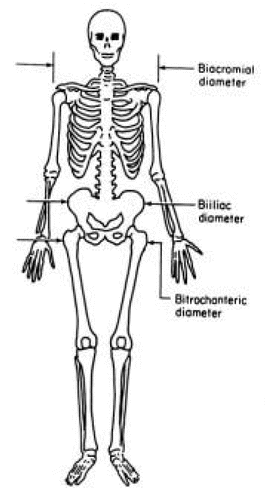{#fig-body-measuresfig-alt="Skeleton of the human body where three variable are measured: The biacromial diameter is the breadth of the shoulder, the biiliac diameter is the pelvic breadth and the bitrochanteric diameter is the breadth of the hip bone."fig-align="center"}To facilitate the following experiment I have written a function to generate a histogram with an overlaid density curve. The code is loaded with other functions whenever this chapter is rendered.:::::{.my-r-code}:::{.my-r-code-header}:::::: {#cnj-chap02-histogram-code}: Function to create histogram with overlaid `dnorm` curve:::::::::::::{.my-r-code-container}```{r}#| label: histogram-code#| eval: false# df = data.frame or tibble# v = numerical column of data.frame: syntax for call df$v# x_label = title for x-axis# nbins = number of bins# col_fill = fill color# col_color = border color of bins# col = color of dnorm curve# return value is "ggplot" object to customize it further (set labels etc.)my_hist_dnorm <-function(df, v, n_bins =20,col_fill ="gray90",col_color ="black",col_dnorm ="tomato") { p <- df |> ggplot2::ggplot(ggplot2::aes()) + ggplot2::geom_histogram( ggplot2::aes(y = ggplot2::after_stat(density)),bins = n_bins,fill = col_fill,color = col_color,stat ="histogram") + ggplot2::stat_function(fun = dnorm,args =c(mean =mean(v),sd =sd(v)),col = col_dnorm) + ggplot2::theme_bw() p}```(*This code chunk is not evaluated and has therefore no visible output.*):::::::::#### Data:::::{.my-r-code}:::{.my-r-code-header}:::::: {#cnj-chap02-load-bdims}: Load the `bdims` dataset of the {**openintro**} package and inspect the data:::::::::::::{.my-r-code-container}```{r}#| label: load-bdimsdata(package ="openintro", list ="bdims")skimr::skim(bdims)```***We can see from the tiny histograms which variable seems to be normally distributed and which are skewed --- and a little less obvious --- which variable has excess kurtosis.:::::::::### Skewness {#sec-chap02-skewness}#### What is skewness?`r glossary("Skewness")` is a measure of the extent to which a distribution is skewed.$$skewness_x = \frac{1}{n}\sum_{i=1}^{n}(\frac{x_i - m_x}{s_x})^3$$ {#eq-chap02-skewness}The mean of $x$, $m_x$, is subtracted from each observation $x_i$. These differences between the mean and each observed value are called `r glossary("deviation scores")`. Each deviation score is divided by the `r glossary("standard deviation")`, $s$, and the result is cubed. Finally, sum the cubed values and divide by the number of cubed values (which is taking the mean) to get the `r glossary("skewness")` of $x$. The resulting value is usually negative when the skew is to the left and usually positive when the skew is toward the right. Skewness is strongly impacted by the sample size, therefore the value of skew that is considered too skewed differs depending on sample size.:::::{.my-assessment}:::{.my-assessment-header}:::::: {#cor-chap02-skewness}: Assessment of skewness:::::::::::::{.my-assessment-container}| Sample Size | Z-values Range | Comment ||----------------|:-------------------------:|---------------------------------|| n < 50 | under -2 or over +2 | Problem! || n > 50 & < 300 | under -3.29 or over +3.29 | Problem! || n > 300 | under -7 or over 7 | Problem, but visual inspection recommended! |: Skewness assessment {#tbl-chap02-skewness} {.striped .hover}- Right skewed = tail to the right = skew index is positive- Left skewed = tail to the left = skew index is negative***:::::::::There are many packages to compute the skewness of a distribution. (Type `??skewness` into the console to get a list. Harris recommends the `skew()` function from the {**semTools**} package (See @sec-semTools). #### Check skewness:::::{.my-experiment}:::{.my-experiment-header}:::::: {#def-check-skewness}: Check skewness of a distribution:::::::::::::{.my-experiment-container}::: {.panel-tabset}###### no skewness:::::{.my-r-code}:::{.my-r-code-header}:::::: {#cnj-chap02-check-male-bia}: Checking skewness of a shoulder breadth distribution of 247 men :::::::::::::{.my-r-code-container}::: {#lst-chap02-check-skew-normal}```{r}#| label: fig-check-skew-normal#| fig-cap: "Shoulder breadth distribution in centimeters of 247 physically active men"#| cache: true#| results: hold## select men from the samplebdims_male <- bdims |> dplyr::filter(sex ==1)## construct graph using my private function my_hist_dnorm()p <-my_hist_dnorm(bdims_male, bdims_male$bia_di)p + ggplot2::labs(x ="biacromial diameter in centimeters")## commented test outputglue::glue("##################################################")glue::glue("Using the `semTools::skew()` function")semTools::skew(bdims_male$bia_di)glue::glue(" ")glue::glue("##################################################")glue::glue("Using the `statpsych::test.skew()` function")statpsych::test.skew(bdims$bia_di)```Checking skewness of a shoulder breadth distribution of 247 men:::*****Interpretation `semTools::skew()`**- **skew (g1)**: `r glossary("Skewness")`- **se**: `r glossary("Standard error")`- **z**: `r glossary("Z-score")`- **p**: `r glossary("p-value")`::: {.callout-tip style="color: darkgreen;"}The interpretation follows @tbl-chap02-skewness: The $z$ result of @fig-check-skew-normal from the biacromial diameter of 247 men is only 1.44, e.g. well situated in the range of -3.29 and +3.29 and therefore we have no skewness problem. The p-value is with 0.17 big and therefore the null (there is no skewness) can't be rejected.:::*****Interpretation `statpsych::test.skew()`**The result of the `statpsych::test.skew()` function is a 1-row matrix:- **Skewness**: Estimate of the `r glossary("skewness")` coefficient- **p**: `r glossary("MCMC", "Monte Carlo")` two-sided `r glossary("p-value")` for test of zero skewness::: {.callout-tip style="color: darkgreen;"}The p-value is way above .05 and therefore the null can't be rejected. e.g., the data is from a normal distribution.:::::::::::::::::{.my-watch-out}:::{.my-watch-out-header}WATCH OUT! Be patienet: Calculation of `statpsych::test.skew()` needs time:::::::{.my-watch-out-container}> [`statpsych::test.skew()` c]omputes a Monte Carlo p-value (250,000 replications) for the null hypothesis that the sample data come from a normal distribution. If the p-value is small (e.g., less than .05) and the skewness estimate is positive, then the normality assumption can be rejected due to positive skewness. If the p-value is small (e.g., less than .05) and the skewness estimate is negative, then the normality assumption can be rejected due to negative skewness. ([R Documentation](https://search.r-project.org/CRAN/refmans/statpsych/html/test.skew.html) of statpsych::test.skew())::::::::::::::{.my-resource}:::{.my-resource-header}:::::: {#lem-chap02-test-normal-dist}Articles on identifying non-normal distributions:::::::::::::{.my-resource-container}Harris referenced [@kim2013] for the assessment table above. I noticed that there are many [short articles about different types of test.](https://synapse.koreamed.org/advanced/index.php). Just put the search string "Statistical[ALL] AND notes[ALL] AND clinical[ALL] AND researchers[ALL]" into the Kamje search engine.:::::::::###### Left skewed:::::{.my-r-code}:::{.my-r-code-header}:::::: {#cnj-chap02-left-skewed}: Pelvic breadth distribution of 507 physically active individuals:::::::::::::{.my-r-code-container}```{r}#| label: fig-check-skew-left#| fig-cap: "Pelvic breadth distribution in centimeters of 507 physically active indidviduals"#| cache: true#| results: hold## construct graph using my private function my_hist_dnorm()p <-my_hist_dnorm(bdims, bdims$bii_di)p + ggplot2::labs(x ="respondent's biiliac diameter (pelvic breadth) in centimeters.")## commented test outputglue::glue("##################################################")glue::glue("Using the `semTools::skew()` function")semTools::skew(bdims$bii_di)glue::glue(" ")glue::glue("##################################################")glue::glue("Using the `statpsych::test.skew()` function")statpsych::test.skew(bdims$bii_di)```***::: {.callout-tip style="color: darkgreen;"}## Skewness interpretation with `semTools::skew()` and `statpsych::test.skew()`Both tests have a very low p-value and attest us excessive skewness. This is even true if the z-value of `semTools::skew()` is only -3.85, e.g. in the appropriate boundaries of -7 and + 7 for a sample of 507 individuals (compare @tbl-chap02-skewness). The recommended visual inspection of the histogram shows us a left skewed distribution: There are too much individuals with a smaller pelvic breadth than it would appropriate for a normal distribution. It is very unlikely that the sample comes from a normal distribution. We have to reject the null.:::@tbl-chap02-skewness:::::::::###### Right skewed:::::{.my-r-code}:::{.my-r-code-header}:::::: {#cnj-chap02-right-skewed}: Waist girth distribution in centimeters of 507 physically active individuals:::::::::::::{.my-r-code-container}```{r}#| label: fig-check-skew-right#| fig-cap: "Waist girth distribution in centimeters of 507 physically active individuals"#| cache: true#| results: hold## construct graph using my private function my_hist_dnorm()p <-my_hist_dnorm(bdims, bdims$wai_gi)p + ggplot2::labs(x ="Respondent's waist girth in centimeters, \nmeasured at the narrowest part of torso below the rib cage as average of contracted and relaxed position")## commented test outputglue::glue("##################################################")glue::glue("Using the `semTools::skew()` function")semTools::skew(bdims$wai_gi)glue::glue(" ")glue::glue("##################################################")glue::glue("Using the `statpsych::test.skew()` function")statpsych::test.skew(bdims$wai_gi)```***::: {.callout-tip style="color: darkgreen;"}## Skewness interpretation with `semTools::skew()` and `statpsych::test.skew()`Both tests have a very low p-value and attest us excessive skewness. Again is the corresponding the z-value of `semTools::skew()` in the appropriate boundaries of -7 and + 7 for a sample of 507 individuals (compare @tbl-chap02-skewness). But the recommended visual inspection of the histogram shows us a right skewed distribution very clearly: There are too much individuals with a bigger waist girth than it would appropriate for a normal distribution. It is very unlikely that the sample comes from a normal distribution. We have to reject the null.::::::::::::::::::::::::### Mode {#sec-chap02-mode}The book claims: "… unfortunately, perhaps because it is rarely used, there is no mode function." This is not correct. There exists {**modeest**}, a package specialized for mode estimation (see @sec-modeest).Harris therefore explains how to sort the variable to get the value most used as first item. This methods works always out of the box and does not need a specialized package.:::::{.my-experiment}:::{.my-experiment-header}:::::: {#def-chap02-mode-estimation}: Estimation of the mode:::::::::::::{.my-experiment-container}::: {.panel-tabset}###### modeest::mfv():::::{.my-r-code}:::{.my-r-code-header}:::::: {#cnj-chap02-mode-mfv}: Most frequent value(s) in a given numerical vector:::::::::::::{.my-r-code-container}```{r}#| label: mode-mfv#| results: holdtr_f <- forcats::fct_count(transgender_pb$TRNSGNDR)tr_recoded <- forcats::fct_count(transgender_clean$TRNSGNDR) |> dplyr::rename(Recoded ="f")tr <- dplyr::full_join(tr_f, tr_recoded, by = dplyr::join_by(n)) |> dplyr::relocate(n, .after = dplyr::last_col())glue::glue("Let's remember the frequencies of the TRNSGNDR variable")trglue::glue(" ")glue::glue("#############################################")glue::glue("TRNSGDR variable not recoded and with NA's")transgender_pb |> dplyr::pull(TRNSGNDR) |> modeest::mfv()glue::glue(" ")glue::glue("#############################################")glue::glue("TRNSGDR variable not recoded with NA's")transgender_pb |> dplyr::pull(TRNSGNDR) |> modeest::mfv(na_rm =TRUE)glue::glue(" ")glue::glue("#############################################")glue::glue("TRNSGDR variable recoded without NA's")transgender_clean |> dplyr::pull(TRNSGNDR) |> modeest::mfv(na_rm =TRUE)```:::::::::The function `mfv()` stands for Most Frequent Value(s) and is reexported by {**modeest**} from {**statip**}. It returns all modes, e.g. highest values from a vector. For instance: `modeest::mfv(c("a", "a", "b", "c", "c"))` returns "`r modeest::mfv(c("a", "a", "b", "c", "c"))`". If you want just the first mode value use `modeest::mfv1()`.###### dplyr::arrange():::::{.my-r-code}:::{.my-r-code-header}:::::: {#cnj-code-name-b}Arrange data that most frequent value(s) are first row:::::::::::::{.my-r-code-container}```{r}#| label: mode-arrange#| results: holdglue::glue("Let's remember the frequencies of the TRNSGNDR variable")trglue::glue(" ")glue::glue("#############################################. ")glue::glue("TRNSGDR variable with NA's")tr |> dplyr::arrange(desc(n)) |> dplyr::dplyr_row_slice(1)glue::glue(" ")glue::glue("#############################################. ")glue::glue("TRNSGDR variable without NA's")tr |> tidyr::drop_na() |> dplyr::arrange(desc(n)) |> dplyr::first()glue::glue(" ")glue::glue("#############################################. ")glue::glue("TRNSGDR variable without NA's: Just the mode value")tr |> tidyr::drop_na() |> dplyr::arrange(desc(n)) |> dplyr::first() |> dplyr::pull(n)```:::::::::::::::::::::### Kurtosis {#sec-chap02-kurtosis}#### What is kurtosis?`r glossary("Kurtosis")` measures how many observations are in the tails of the distribution. If a distribution that looks bell-shaped has many observations in the tails it is more flat than a normal distribution and called `r glossary("platykurtic")`. On the other hand if a distribution has that looks bell-shaped has only a few observations in the tails it is more pointy than a normal distribution and called `r glossary("leptokurtic")`. A normal distribution is `r glossary("mesokurtic")`, e.g., it is neither platykurtic nor leptokurtic.Platykurtic and leptokurtic deviations from normality do not necessarily influence the `r glossary("Arithmetic Mean", "mean")`, since it will still be a good representation of the middle of the data if the distribution is symmetrical and not `r glossary("skewness", "skewed")`. However, platykurtic and leptokurtic distributions will have smaller and larger values of `r glossary("variance var", "variance")` and `r glossary("standard deviation")`, respectively, compared to a normal distribution. And this is a problem, as variance and standard deviation are not only used to quantify spread, but are also used in many of the common statistical tests.***$$kurtosis_{n} = \frac{1}{n}\sum_{i=1}^{n}(\frac{x_i - m_x}{s_x})^4$$ {#eq-chap02-kurtosis}- $n$: Sample size- $s_{x}$: Standard deviation- $m_{x}$: The mean of $x$- $x_{i}$: Each value of $x$***:::::{.my-assessment}:::{.my-assessment-header}:::::: {#cor-chap02-kurtosis}: How to evaluate kurtosis?:::::::::::::{.my-assessment-container}| kurtosis (z) value | Compared to normal distribution ||:-------------------------:|---------------------------------|| around 3 | Normal distribution (mesokurtic) || above 3 | Less observations in tails (leptokurtic, pointy) || below 3 | More observation in tails (platykurtic, flat) |: Kurtosis assessment {#tbl-chap02-kurtosis} {.striped .hover}:::::::::#### Check excess of kurtosis:::::{.my-experiment}:::{.my-experiment-header}:::::: {#def-chap02-check-kurtosis}: Check excess of kurtosis:::::::::::::{.my-experiment-container}::: {.panel-tabset}###### no kurtosis:::::{.my-r-code}:::{.my-r-code-header}:::::: {#cnj-chap02-check-kurtosis-normal}: Checking kurtosis of hip girth distribution of 507 individuals:::::::::::::{.my-r-code-container}```{r}#| label: fig-check-kurtosis-normal#| fig-cap: "Respondent's bitrochanteric diameter (hip girth) in centimeters of 507 individuals"#| cache: true#| results: hold## construct graph using my private function my_hist_dnorm()p <-my_hist_dnorm(bdims, bdims$bit_di)p + ggplot2::labs(x ="respondent's bitrochanteric diameter (hip girth) in centimeters of 507 individuals")glue::glue("###################################################################")glue::glue("Kurtosis of pelvic breadth using `semTools::kurtosis()`")semTools::kurtosis(bdims$bit_di)glue::glue(" ")glue::glue("###################################################################")glue::glue("Kurtosis of pelvic breadth using `statpsych::test.kurtosis()`")statpsych::test.kurtosis(bdims$bit_di)```***The excessive kurtosis computed by default is $g_{2}$, the fourth standardized moment of the empirical distribution.***::: {.callout-tip style="color: darkgreen;"}## Kurtosis test of the pelvic breadth distributionBoth functions `semTools::skew()` and `statpsych::test.skew()` claim that there is no excess kurtosis. The z-value is small and the p-value is high, so we don't have to reject the null: The probability is very high, that the data come from a normal distribution.::::::::::::###### Platykurtic (flat):::::{.my-r-code}:::{.my-r-code-header}:::::: {#cnj-chap02-check-kurtosis-flat}: Checking kurtosis of shoulder breadth distribution of 507 individuals:::::::::::::{.my-r-code-container}```{r}#| label: fig-check-kurtosis-flat#| fig-cap: "Biachromial diameter (shoulder breadth) distribution of 507 individuals"#| cache: true#| results: hold## construct graph using my private function my_hist_dnorm()p <-my_hist_dnorm(bdims, bdims$bia_di)p + ggplot2::labs(x ="biachromial diameter distribution of 507 individuals")glue::glue("###################################################################")glue::glue("Kurtosis of biachromial diameter using `semTools::kurtosis()`")semTools::kurtosis(bdims$bia_di)glue::glue(" ")glue::glue("###################################################################")glue::glue("Kurtosis of biachromial diameter using `statpsych::test.kurtosis()`")statpsych::test.kurtosis(bdims$bia_di)```***::: {.callout-tip style="color: darkgreen;"}## Kurtosis test of the shoulder breadth distributionBoth functions `semTools::skew()` and `statpsych::test.skew()` assert that there is excess kurtosis. The p-value is very low, so we have to reject the null and assuming the alternative: The probability is very high, that the data didn't come from a normal distribution.As the z-value is below 3 and the excess value is negative we have a platykurtic (= flat) distribution. Looking at the histogram shows that this a reasonable interpretation.::::::::::::###### Leptokurtic (pointy):::::{.my-r-code}:::{.my-r-code-header}:::::: {#cnj-chap02-check-kurtosis-pointy}: Checking kurtosis of pelvis breadth distribution of 507 individuals:::::::::::::{.my-r-code-container}```{r}#| label: fig-check-kurtosis-pointy#| fig-cap: "Respondent's biiliac diameter (pelvic breadth) in centimeters of 507 individuals"#| results: hold#| cache: true## construct graph using my private function my_hist_dnorm()p <-my_hist_dnorm(bdims, bdims$bii_di)p + ggplot2::labs(x ="Respondent's biiliac diameter (pelvic breadth) in centimeters (men and women, N = 507)")glue::glue("###################################################################")glue::glue("Kurtosis of pelvis breadth distribution using `semTools::kurtosis()`")semTools::kurtosis(bdims$bii_di)glue::glue(" ")glue::glue("###################################################################")glue::glue("Kurtosis of pelvis breadth distribution using `statpsych::test.kurtosis()`")statpsych::test.kurtosis(bdims$bii_di)```***::: {.callout-tip style="color: darkgreen;"}## Kurtosis test of the height distributionBoth functions `semTools::skew()` and `statpsych::test.skew()` assert that there is excess kurtosis. The p-value is very low, so we have to reject the null and assuming the alternative: The probability is very high, that the data didn't come from a normal distribution.As the z-value is above 3 and the excess value is positive we have a leptokurtic (= pointy) distribution. Looking at the histogram shows that this a reasonable interpretation.:::::::::::::::::::::::::::::{.my-important}:::{.my-important-header}Using only {**semTools**} for testing skewness and kurtosis:::::::{.my-important-container}I haven't found any difference between the results of {**semTools**} and {**statpsych**} in the computation of skewness and kurtosis. As the {**statpsych**} is more cumbersome, because of its 250,000 replications, I will stick with the {**semTools**} functions.:::::::::***### Scientifc notationI have not troubles to read figures in `r glossary("scientific notation")`. But I often forget what command I must use to turn it off/on.- To turn off this option in R, type and run `options(scipen = 999)`. - To turn it back on, type and run `options(scipen = 000)`.- For graphs you could change the scale of the axis:```ggplot(aes(x = Year, y = num.guns/100000)) + geom_line(aes(color = gun.type)) +labs(y = "Number of firearms (in 100,000s)")```- To turn off just for one variable: `format(x, scientific = FALSE)`. It returns a character vector.### Data management for numerical variables#### The book's `PHYSHLTH` variable:::::{.my-example}:::{.my-example-header}:::::: {#exm-chap02-data-wrangling-numerical}: Data management for numerical `PHYSHLTH` variable:::::::::::::{.my-example-container}::: {.panel-tabset}###### Codebook:::::{.my-r-code}:::{.my-r-code-header}:::::: {#cnj-chap02-codebook-physical-health}Find numerical variable `PHYSHLTH` in codebook :::::::::::::{.my-r-code-container}```{r}#| label: select-physical-health#| results: holdbrfss_tg_2014 <- base::readRDS("data/chap02/brfss_tg_2014_raw.rds")physical_health <- brfss_tg_2014 |> dplyr::select(PHYSHLTH)utils::str(physical_health)base::summary(physical_health)skimr::skim(physical_health)```***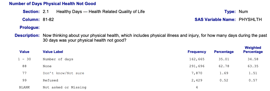{#fig-physical-health-codebookfig-alt="Table about health status from BEHAVIORAL RISK FACTOR SURVEILLANCE SYSTEMCODEBOOK REPORT (BRFSS), 2014" fig-align="center"}***:::::::::###### Recode:::::{.my-r-code}:::{.my-r-code-header}:::::: {#cnj-chap02-recode-physical-health}Recode numerical variable `PHYSHLTH`:::::::::::::{.my-r-code-container}```{r}#| label: recode-physical-health#| results: holdphysical_health_clean <- physical_health |> dplyr::mutate(PHYSHLTH = dplyr::case_match(PHYSHLTH, 77~NA,99~NA,88~0,.default = PHYSHLTH))base::summary(physical_health_clean)skimr::skim(physical_health_clean)```:::::::::###### Histogram:::::{.my-r-code}:::{.my-r-code-header}:::::: {#cnj-chap02-histogram-physical-health}: Plot histogram of numerical variable `PHYSHLTH`:::::::::::::{.my-r-code-container}{#lst-chap02-histogram-physical-health}```{r}#| label: fig-histogram-physical-health#| fig-cap: "Number of days where physical health is not good"physical_health_clean |> ggplot2::ggplot(ggplot2::aes(x = PHYSHLTH)) + ggplot2::geom_histogram(binwidth =1, na.rm =TRUE) + ggplot2::scale_y_continuous(labels =function(x){ trans = x /1000; base::paste0(trans, "K") }) +# ggplot2::scale_y_continuous(labels = scales::label_number()) + ggplot2::theme_bw()```Number of days where physical health is not good:::::::::::::::::{.my-remark}:::{.my-remark-header}Two code changes compared to the books code chunk for figure 2.9:::::::{.my-remark-container}**1. Preventing warning messages**I added `binwidth = 1, na.rm = TRUE` into the `ggplot2::geom_histogram()` function to prevent two warning messages:> - Warning: `stat_bin()` using `bins = 30`. Pick better value with `binwidth`.> - Warning: Removed 10303 rows containing non-finite values (`stat_bin()`).Concerning the first warning: `bins = 30` wouldn't be ideal, because we have 31 values (0-30 days where the physical health was not good). So `bins = 31` would also be a good choice.I have to confess that I didn't know that one can use the argument `na.rm = TRUE` inside a {**ggplot2**} function.**2. Removing the scientific notation in the y-axis**- At first I used used outside the {**ggplot2**}-block options(scipen = 999)`. But then I decided not to turn off generally the scientific notation but to find a solution inside of the {**ggplot2**} code chunk. - I came up with `ggplot2::scale_y_continuous(labels = scales::label_number())`. Using the {**scales**} package is a common way to change scales and labels of {**ggplot2**} graphics (see @sec-scales). My command changed the scientific notation to numbers, but the numbers still had many zeros and are not handy.- Finally I found a general solution, without using the {**scales**} package: Writing a local function for the `trans` argument of the `ggplot2::scale_y_continuous()` directive. I didn't know about this method before and found this solution on [StackOverflow](https://stackoverflow.com/questions/44656907/scale-y-continious-divide-by-1-000-and-append-k).:::::::::###### Central tendency:::::{.my-r-code}:::{.my-r-code-header}:::::: {#cnj-chap02-central-tendency-physhlth}: Computing mean, median and mode of the `PHYSHLTH` variable:::::::::::::{.my-r-code-container}```{r}#| label: central-tendency-physhlthphysical_health_clean |> tidyr::drop_na() |> dplyr::summarize(mean = base::mean(PHYSHLTH),median = stats::median(PHYSHLTH),mode = modeest::mfv(PHYSHLTH))```:::::::::###### Spread:::::{.my-r-code}:::{.my-r-code-header}:::::: {#cnj-chap02-spread-physhlth}: Computing standard deviation, variance, the IQR and the qunatiles of the `PHYSHLTH` variable:::::::::::::{.my-r-code-container}```{r}#| label: spread-physhlth#| results: holdphysical_health_clean |> tidyr::drop_na() |> dplyr::summarize(sd = stats::sd(PHYSHLTH),var = stats::var(PHYSHLTH),IQR = stats::IQR(PHYSHLTH) )glue::glue(" quantiles corresponding to the given probabilities")stats::quantile(physical_health_clean$PHYSHLTH, na.rm =TRUE)```:::::::::::::::::::::#### Achievement 3: The `_AGE80` variable:::::{.my-exercise}:::{.my-exercise-header}:::::: {#exr-chap02-achievement-3}: Data management with the `_AGE80` variable:::::::::::::{.my-exercise-container}::: {.panel-tabset}###### Codebook & Summary:::::{.my-r-code}:::{.my-r-code-header}:::::: {#cnj-chap02-codebook-age80}: Get Codebook and first summary of raw data:::::::::::::{.my-r-code-container}```{r}#| label: codebook-age80#| results: holdbrfss_tg_2014 <- base::readRDS("data/chap02/brfss_tg_2014_raw.rds")age80 <- brfss_tg_2014 |> dplyr::select(`_AGE80`)utils::str(age80)skimr::skim(age80)base::summary(age80)```***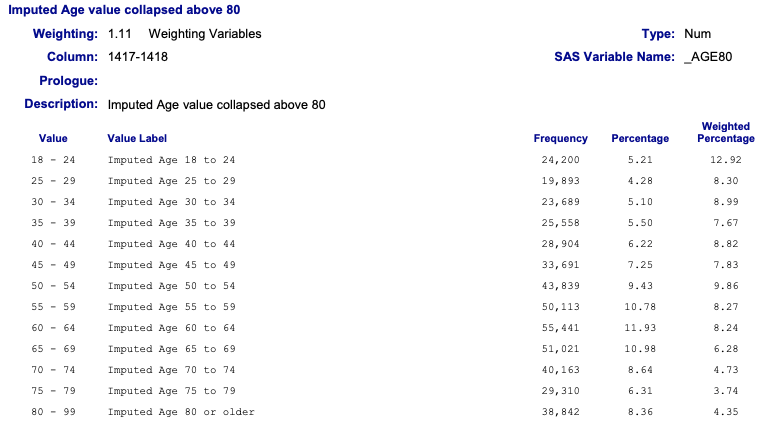{#fig-age80-codebookfig-alt="Imputed Age value collapsed above 80"fig-align="center"}***Remember: I have used as column name `_AGE80` (and not `X_AGE80`) when I imported with {**haven**} the data in @lst-chap02-get-brfss-2014-data.The age of the respondents range from 18 to 80. **The good news**: There are no missing values or other codes that we need to recode.**The bad news**: The age value of 80 includes all people 80 and above. Therefore age 80 will have more observations as it would be appropriate for this age. As a consequence we can expect that the age distribution would be biased to the right (= left skewed). This is confirmed in two ways: (1) The median is higher than the mean and (2) we see the left skewed distribution also in the tiny histogram from the `skimr::skim()` summary.:::::::::###### _AGE80 measures:::::{.my-r-code}:::{.my-r-code-header}:::::: {#cnj-chap02-age80-measures}: Central tendency, spread, skewness & kurtosis of `_AGE80`:::::::::::::{.my-r-code-container}```{r}#| label: tbl-age80-measures#| tbl-cap: "Age distribution of 464664 individuals (age value collapsed above 80)"#| results: holdglue::glue("###################################################################")glue::glue("Central tendency and spread measures of `_AGE80` variable")age80 |> dplyr::summarize(mean = base::mean(`_AGE80`), median = stats::median(`_AGE80`), mode = modeest::mfv(`_AGE80`),min = base::min(`_AGE80`),max = base::max(`_AGE80`),sd = stats::sd(`_AGE80`),var = stats::var(`_AGE80`),IQR = stats::IQR(`_AGE80`) )## construct graph using my private function my_hist_dnorm()p <-my_hist_dnorm(age80, age80$`_AGE80`, n_bins =62)p + ggplot2::labs(x ="Age distribution of 464664 individuals (age value collapsed above 80)") + ggplot2::scale_x_continuous(breaks =seq(20,80,10))glue::glue(" ")glue::glue("###################################################################")glue::glue("Skewness of `_AGE80` variable")semTools::skew(age80$`_AGE80`)glue::glue(" ")glue::glue("###################################################################")glue::glue("Kurtosis of `_AGE80` variable")semTools::kurtosis(age80$`_AGE80`)```***Instead of `base::range()` I have used `base::min()` and `base::max()`.As we already have assumed from the over sized 80 year value we have a left skewed distribution. But we have also excess kurtosis, because we have to much observation in the tails, e.g., the distribution is too flat (platykurtic) to come from a normal distribution.Now lets see the values after we have removed the obvious bias with the 80 year value. We will generate a new variable `_AGE79` that range only from 18 to 79 years.:::::::::###### _AGE79 measures:::::{.my-r-code}:::{.my-r-code-header}:::::: {#cnj-chap02-age79-measures}: Central tendency, spread, skewness & kurtosis of `_AGE79`:::::::::::::{.my-r-code-container}```{r}#| label: tbl-age79-measures#| tbl-cap: "Age distribution of 425822 individuals from age 18 to 79"#| results: holdglue::glue("###################################################################")glue::glue("Central tendency and spread measures of `_AGE79` variable")age79 <- age80 |> dplyr::filter(`_AGE80`<=79) |> dplyr::rename(`_AGE79`=`_AGE80`)age79 |> dplyr::summarize(mean = base::mean(`_AGE79`), median = stats::median(`_AGE79`), mode = modeest::mfv(`_AGE79`),min = base::min(`_AGE79`),max = base::max(`_AGE79`),sd = stats::sd(`_AGE79`),var = stats::var(`_AGE79`),IQR = stats::IQR(`_AGE79`) )## construct graph using my private function my_hist_dnorm()p <-my_hist_dnorm(age79, age79$`_AGE79`, n_bins =61)p + ggplot2::labs(x ="Age distribution of 425822 individuals from age 18 to 79") + ggplot2::scale_x_continuous(breaks =seq(20,80,10))glue::glue(" ")glue::glue("###################################################################")glue::glue("Skewness of `_AGE79` variable")semTools::skew(age79$`_AGE79`)glue::glue(" ")glue::glue("###################################################################")glue::glue("Kurtosis of `_AGE79` variable")semTools::kurtosis(age79$`_AGE79`)```***Filtering the data to get only values between 18-79 doesn't normalize the distribution. We can clearly see that there are too many people between 58 to 74 years respectively there is a gap in the cohorts from 35 to 55 years.:::::::::::::::::::::***## Creating tables for publishing {#sec-chap02-create-tables-for-publishing}### Necessary featuresWe need to manipulate data to provide a table with all its requiredfeatures as they are:::: {#bul-chap02-table-features}:::::{.my-bullet-list}:::{.my-bullet-list-header}Bullet List:::::::{.my-bullet-list-container}1. A main title indicating what is in the table, including - the overall sample size - key pieces of information that describe the data such as the year of data collection and the data source - the units of measurement (people, organizations, etc.) 2. Correct formatting, including - consistent use of the same number of decimal places throughout the table - numbers aligned to the right so that the decimal points line up - words aligned to the left- indentation and shading to differentiate rows or sections3. Clear column and row labels that have - logical row and column names - a clear indication of what the data are, such as means or frequencies - row and column sample sizes when they are different from overall sample sizes [@harris2020].:::::::::Required features of a table:::***The table I am going to reproduce: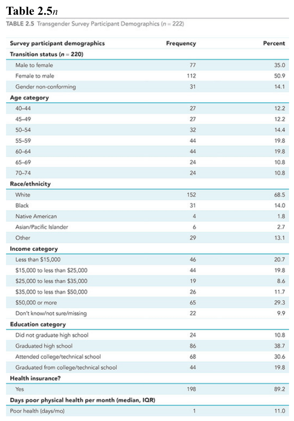{#fig-table1-example2fig-alt="Transgender Survey Participants Demographics (n = 220)"fig-align="center"}### Table generation step-by-stepI will use Table 2.5 (here it is @fig-table1-example2) from the book as my goal model that I want to replicate. In my first approach I will use {**gtsummary**} and document every step of the development process.:::::{.my-example}:::{.my-example-header}:::::: {#exm-chap02-table-generation}: replication:::::::::::::{.my-example-container}::: {.panel-tabset}###### Filter & Select:::::{.my-r-code}:::{.my-r-code-header}:::::: {#cnj-code-name-a}: Filter and Select:::::::::::::{.my-r-code-container}```{r}#| label: table1-step1brfss_tg_2014 <- base::readRDS("data/chap02/brfss_tg_2014_raw.rds")brfss_2014_raw <- brfss_tg_2014 |> tidyr::drop_na() |> dplyr::filter(TRNSGNDR <=3) |> dplyr::filter(`_AGEG5YR`>=5&`_AGEG5YR`<=11) |> dplyr::select(-c(HADMAM, `_AGE80`))utils::str(brfss_2014_raw)skimr::skim(brfss_2014_raw)```***As first step I have reduced the dataset to those categories that are outlined in @fig-table1-example2. We will work with 222 records, 2 more as in the model table data are mentioned. But in the header it says "(n = 222)".:::::::::###### Recode:::::{.my-r-code}:::{.my-r-code-header}:::::: {#cnj-chap2-table-recode}Recode:::::::::::::{.my-r-code-container}```{r}#| label: text-bbrfss_2014_recoded <- brfss_2014_raw |> dplyr::mutate(TRNSGNDR = forcats::as_factor(TRNSGNDR)) |> dplyr::mutate(TRNSGNDR = forcats::fct_recode(TRNSGNDR, "Male to female"="1")) |> dplyr::mutate(TRNSGNDR = forcats::fct_recode(TRNSGNDR, "Female to male"="2")) |> dplyr::mutate(TRNSGNDR = forcats::fct_recode(TRNSGNDR, "Gender non-conforming"="3")) |> dplyr::mutate(`_AGEG5YR`= forcats::as_factor(`_AGEG5YR`)) |> dplyr::mutate(`_AGEG5YR`= forcats::fct_recode(`_AGEG5YR`, "40-44"="5")) |> dplyr::mutate(`_AGEG5YR`= forcats::fct_recode(`_AGEG5YR`, "45-49"="6")) |> dplyr::mutate(`_AGEG5YR`= forcats::fct_recode(`_AGEG5YR`, "50-54"="7")) |> dplyr::mutate(`_AGEG5YR`= forcats::fct_recode(`_AGEG5YR`, "55-59"="8")) |> dplyr::mutate(`_AGEG5YR`= forcats::fct_recode(`_AGEG5YR`, "60-64"="9")) |> dplyr::mutate(`_AGEG5YR`= forcats::fct_recode(`_AGEG5YR`, "65-69"="10")) |> dplyr::mutate(`_AGEG5YR`= forcats::fct_recode(`_AGEG5YR`, "70-74"="11")) |> dplyr::mutate(`_RACE`= forcats::as_factor(`_RACE`)) |> dplyr::mutate(`_RACE`= forcats::fct_recode(`_RACE`, "White"="1")) |> dplyr::mutate(`_RACE`= forcats::fct_recode(`_RACE`, "Black"="2")) |> dplyr::mutate(`_RACE`= forcats::fct_recode(`_RACE`, "Native American"="3")) |> dplyr::mutate(`_RACE`= forcats::fct_recode(`_RACE`, "Asian/Pacific Islander"="4")) |> dplyr::mutate(`_RACE`= forcats::fct_collapse(`_RACE`, "Other"=c("5", "7", "8", "9"))) |> dplyr::mutate(`_INCOMG`= forcats::as_factor(`_INCOMG`)) |> dplyr::mutate(`_INCOMG`= forcats::fct_recode(`_INCOMG`, "Less than $15,000"="1")) |> dplyr::mutate(`_INCOMG`= forcats::fct_recode(`_INCOMG`, "$15,000 to less than $25,000"="2")) |> dplyr::mutate(`_INCOMG`= forcats::fct_recode(`_INCOMG`, "$25,000 to less than $35,000"="3")) |> dplyr::mutate(`_INCOMG`= forcats::fct_recode(`_INCOMG`, "$35,000 to less than $50,000"="4")) |> dplyr::mutate(`_INCOMG`= forcats::fct_recode(`_INCOMG`, "$50,000 or more"="5")) |> dplyr::mutate(`_INCOMG`= forcats::fct_recode(`_INCOMG`, "Don't know/not sure/missing"="9")) |> dplyr::mutate(`_EDUCAG`= forcats::as_factor(`_EDUCAG`)) |> dplyr::mutate(`_EDUCAG`= forcats::fct_recode(`_EDUCAG`, "Did not graduate highschool"="1")) |> dplyr::mutate(`_EDUCAG`= forcats::fct_recode(`_EDUCAG`, "Graduated highschool"="2")) |> dplyr::mutate(`_EDUCAG`= forcats::fct_recode(`_EDUCAG`, "Attended college/technical school"="3")) |> dplyr::mutate(`_EDUCAG`= forcats::fct_recode(`_EDUCAG`, "Graduated from college/technical school"="4")) |> dplyr::mutate(HLTHPLN1 = forcats::as_factor(HLTHPLN1)) |> dplyr::mutate(HLTHPLN1 = forcats::fct_recode(HLTHPLN1, "Yes"="1")) |> dplyr::mutate(HLTHPLN1 = forcats::fct_recode(HLTHPLN1, "No"="2")) |> dplyr::mutate(PHYSHLTH = dplyr::case_match(PHYSHLTH, 77~NA,99~NA,88~0,.default = PHYSHLTH)) |> labelled::set_variable_labels(TRNSGNDR ="Transition status",`_AGEG5YR`="Age category",`_RACE`="Race/ethnicity",`_INCOMG`="Income category",`_EDUCAG`="Education category",HLTHPLN1 ="Health insurance?",PHYSHLTH ="Days poor physical health per month" )```:::::{.my-watch-out}:::{.my-watch-out-header}WATCH OUT! Warning because of missing level `6` in `_RACE` variable:::::::{.my-watch-out-container}In my first run of this long R code I got the following warning:> - Warning: There was 1 warning in `dplyr::mutate()`.> - ℹ In argument: `_RACE = forcats::fct_collapse(...)`.> - Caused by warning:> - ! Unknown levels in `f`: 6No big deal, but to prevent this warning I didn't collapse this level into "Other" in the following runs.::::::::::::::::::###### 1st try:::::{.my-r-code}:::{.my-r-code-header}:::::: {#cnj-chap02-table1-1st-try}: Transgender Survey Participants Demographics (1st try):::::::::::::{.my-r-code-container}```{r}#| label: tbl-table1-1st-try#| tbl-cap: "Transgender Survey Participants Demographics"#| brfss_2014_recoded |> gtsummary::tbl_summary()```:::::::::My first try for a table 1 was just a one-liner with `gtsummary::tbl_summary()`. It looks already pretty good. But let's compare with @fig-table1-example2 in detail:1. My version is different in the header. It has "Characteristics" instead of "Survey participants demographics" and "N = 222" instead of "Frequency" and "Percentage" as separated columns.2. My percentage values do not have one decimal place.3. It is not obvious to which variable the "median, (IQR)" footnote belongs.4. My labels are not bold.I am not sure if I should account also for another difference: My "Health insurance" does not show the value "Yes" in a separate line. The same happens with "Days of poor physical health per month". But I believe that my version is better as it prevents to show redundant information. My separate last line "Unknown" is in any case better, because it is an important information.The first difference may be challenged for the same reason: Including "Frequency" and (braced) "Percentage" in one column and explained by a footnote is practically the same information just more compressed. It would provide more space for further information for more complex tables. So I will concentrate on number (2) to (4) and change in (1) only "Characteristic" to "Survey participants demographics".###### Final 1:::::{.my-r-code}:::{.my-r-code-header}:::::: {#cnj-chap02-table1-2nd-try}: Transgender Survey Participants Demographics (2nd try):::::::::::::{.my-r-code-container}```{r}#| label: tbl-table1-2nd-try#| tbl-cap: "Transgender Survey Participants Demographics"#| cache: truebrfss_2014_gtsummary <- brfss_2014_recoded |> gtsummary::tbl_summary(digits =list(gtsummary::all_categorical() ~c(0, 1)),label = PHYSHLTH ~"Days poor physical health per month (median, IQR)" ) |> gtsummary::bold_labels() |> gtsummary::modify_header(label ="**Survey participants demographics**",stat_0 ="**N = {n} ({style_percent(p)}%)**" ) brfss_2014_gtsummary```:::::::::This would be the final result adapted to the features and possibilities of {**gtsummary**}. But just for the sake of learn more about {**gtsummary**} let's separate frequencies and percent values into two columns. The [advice in StackOverflow](https://stackoverflow.com/questions/68687297/split-frequency-and-percentage-in-tbl-summary-in-to-two-separate-columns) is to generate two table objects with the standard `gtsummary::tbl_summary()` and then to merge them with `gtsummary::tbl:merge()`.###### Final 2:::::{.my-r-code}:::{.my-r-code-header}:::::: {#cnj-chap02-table1-3rd-try}: Transgender Survey Participants Demographics (3rd try):::::::::::::{.my-r-code-container}```{r}#| label: tbl-table1-3rd-try#| tbl-cap: "Transgender Survey Participants Demographics"#| cache: truetbl1_gtsummary <- brfss_2014_recoded |> gtsummary::tbl_summary(statistic =list( gtsummary::all_continuous() ~"{median}", gtsummary::all_categorical() ~"{n}" ), label = PHYSHLTH ~"Days poor physical health per month (median, IQR)" )tbl2_gtsummary <- brfss_2014_recoded |> gtsummary::tbl_summary(statistic =list( gtsummary::all_continuous() ~"({p25}, {p75})", gtsummary::all_categorical() ~"{p}%" ),digits =list(gtsummary::all_categorical() ~1),label = PHYSHLTH ~"Days poor physical health per month (median, IQR)" )tbl_merge_gtsummary <- gtsummary::tbl_merge(list(tbl1_gtsummary, tbl2_gtsummary)) |> gtsummary::bold_labels() |> gtsummary::modify_header(list( label ~"**Survey participants demographics (N = {n})**", stat_0_1 ~"**Frequency**", stat_0_2 ~"**Percent**" ) ) |> gtsummary::modify_spanning_header(gtsummary::everything() ~NA) |> gtsummary::modify_footnote(gtsummary::everything() ~NA) tbl_merge_gtsummary```:::::::::The separation of the frequencies and percentages into two columns worked. But now we have an unfavorable line break in the first column with the variable labels. The problem is that the space between the columns are to wide, especially between second and third column.I couldn't find a way to reduce the space between columns. Maybe I would need to generate a new theme. But I have chosen to other possibilities: - choosing a smaller font- choosing a more compact display###### Small:::::{.my-r-code}:::{.my-r-code-header}:::::: {#cnj-ID-text}: Numbered R Code Title:::::::::::::{.my-r-code-container}```{r}#| label: code-chunk-nametbl_merge_gtsummary_small <- tbl_merge_gtsummary |> gtsummary::as_gt() |> gt::tab_options(table.font.size ="14px")tbl_merge_gtsummary_small```:::::::::The trick to get these details is to convert the {**gtsummary**} object with `gtsummary::as_gt()` into a {**gt**} object and then change the relevant characteristic. {**gt**} has much more control over the table display then {**gtsummary**} which has its strength to calculate and display values in a predefined `r glossary("table 1")` style.{**gtsummary**} has [several themes](https://www.danieldsjoberg.com/gtsummary/reference/theme_gtsummary.html) and support also different languages. But it is possible to [write your own theme](https://www.danieldsjoberg.com/gtsummary/articles/themes.html#writing-themes).###### Compact:::::{.my-r-code}:::{.my-r-code-header}:::::: {#cnj-ID-text}: Numbered R Code Title:::::::::::::{.my-r-code-container}```{r}#| label: code-chunk-name2#| results: holdgtsummary::theme_gtsummary_compact() tbl_merge_gtsummary```:::::::::Here I have used the predefined compact theme with reduced font size and smaller cell paddings.::::::::::::***## Exercises (empty)I have skipped the chapter exercises: They bring nothing new for me. I have already done the recoding and table construction extensively and feel secure about these data management tasks.## Glossary```{r}#| label: glossary-table#| echo: falseglossary_table()```------------------------------------------------------------------------## Session Info {.unnumbered}::: my-r-code::: my-r-code-headerSession Info:::::: my-r-code-container```{r}#| label: session-infosessioninfo::session_info()```::::::