Chapter 5 Missing data Patterns
To get an idea about the complexity of the missing data problem in your dataset and information about the location of the missing values, the missing data pattern can be evaluated.
5.1 Missing data patterns in SPSS
We use the options of the Missing Value Analysis (MVA) procedure in SPSS (Hill (n.d.)). The example dataset contains information on 9 study variables for 150 back pain patients. The continuous variables are Pain, Tampa scale, Disability, Body weight, Body length and Age. The dichotomous variables are Radiation in the leg, Smoking, and Gender. Only the variables Gender and Age are completely observed.
To access the MVA function in the SPSS menu choose:
Analyze -> Missing Value Analysis…
In this menu, transfer all continuous variables to the Quantitative variables window and the categorical variables to the Categorical variables window. Then select the Patterns option. From the Patterns menu (Figure 5.1 select the options Tabulated cases, grouped by missing value patterns and sort variables by missing value pattern. To obtain the full list of all patterns that occur in the data, set the “Omit patterns with less than 1% of cases” at 0%, then click continue and OK.
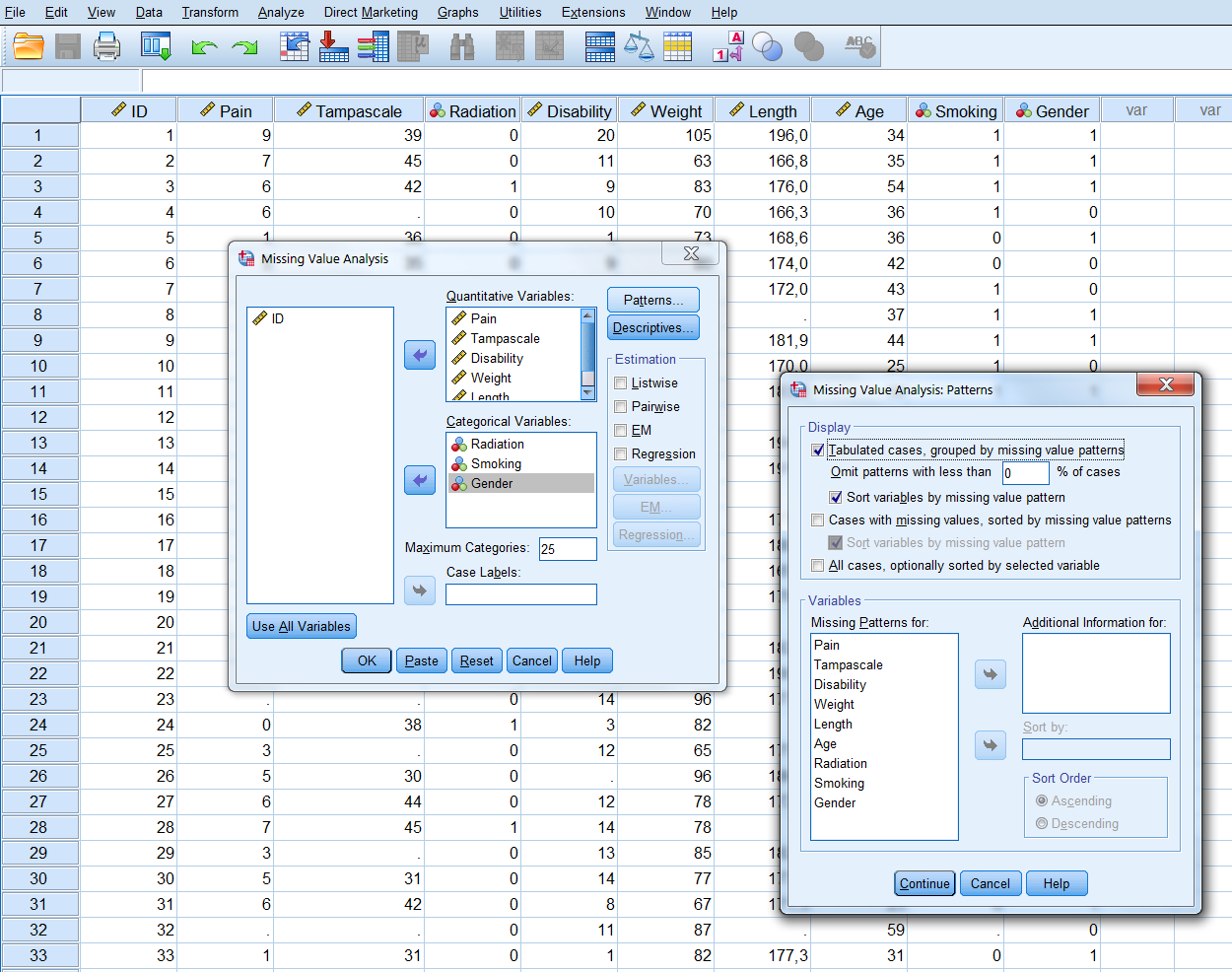
Figure 5.1: The Patterns menu
By default, univariate statistics are presented that include output information about the number and percentages of missing data and descriptive statistics for each variable (Figure 5.2).
Information about the missing data patterns is provided in the Tabulated patterns table. On the left column of that table, named “Number of Cases”, the number of cases are presented with that specific missing data pattern. In our example, there are 75 cases without any missing value and 13 cases with a missing value in only the Tampa scale variable (see row 1 and 2 in (Figure 5.2). In the right column of that table named “Complete if…”, the total number of subjects is presented if the variables that contain missing data in that pattern are not used in the analysis. Those variables are marked with the “X” symbol. For example, 88 subjects remain in the analysis when the variable tampa scale is not used in the analysis, these are the 75 subjects that have completely observed data on top of the 13 subjects with missing data in the Tampa scale variable only.
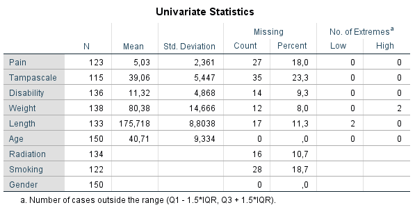
Figure 5.2: Descriptive missing data statistics and the missing data patterns.
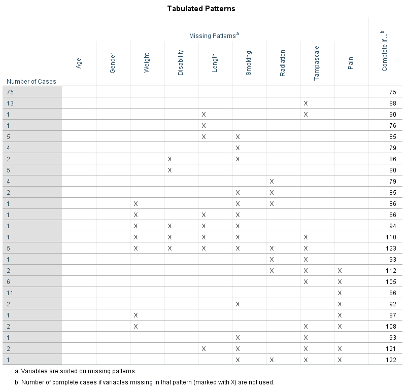
Figure 5.2: Descriptive missing data statistics and the missing data patterns.
Another way to obtain information about the missing data patterns is by accessing the Multiple Imputation menu option. To access this menu, choose:
Analyze -> Multiple Imputation -> Analyze Patterns…
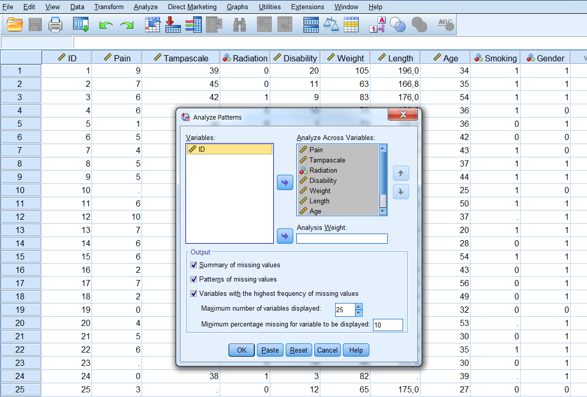
Figure 5.3: Analyse Patterns menu.
Now transfer all variables for the missing value analysis to the window “Analyze Across Variables”. The following output options can be selected:
- Summary of missing values: displays missing data information in pie charts, Patterns of missing values (displays tabulated patterns of missing values.
- Variables with the highest frequency of missing values: displays a table of analysis variables sorted by percent of missing values in decreasing order. .
- Minimum percentage missing for varaibles to be displayed: set at 0 to obtain the full list of all patterns.
- Adjust the maximum number of variables displayed.
The following output will be displayed after selecting all options:
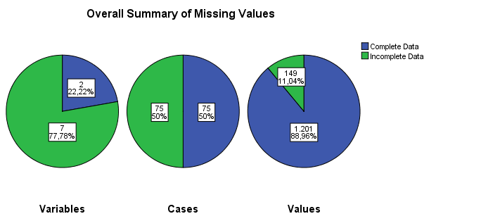
Figure 5.4: Output as a result of the Analyze Patterns menu under Multiple Imputation.
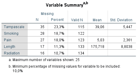
Figure 5.4: Output as a result of the Analyze Patterns menu under Multiple Imputation.
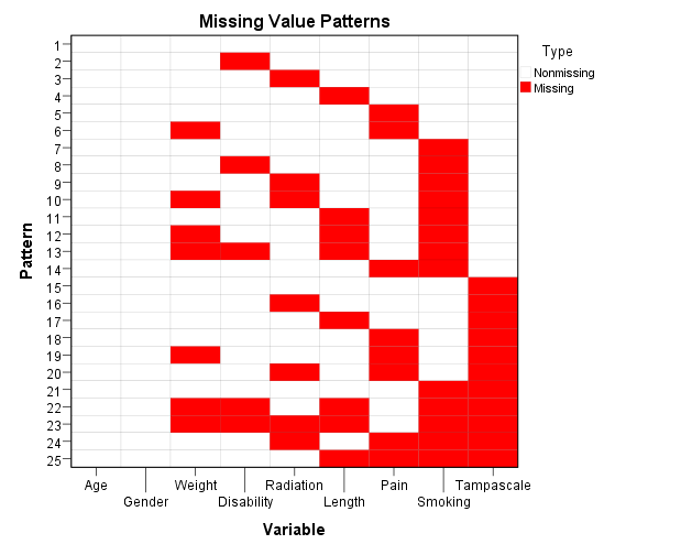
Figure 5.4: Output as a result of the Analyze Patterns menu under Multiple Imputation.
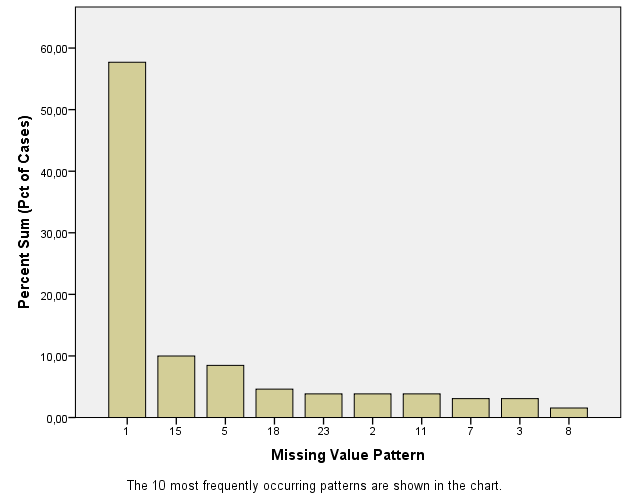
Figure 5.4: Output as a result of the Analyze Patterns menu under Multiple Imputation.
5.2 Missing data patterns in R
To display the missing data patterns in R we can use the mice or VIM package. We start with the mice package. This package contains the md.pattern function that produces the missing data pattern.

##    ID Pain Tampascale Disability Radiation Gender GA
## 21  1    1          1          1         1      1  1  0
## 29  1    1          1          1         1      1  0  1
##     0    0          0          0         0      0 29 29
The first row contains the variable names. Each other row represents a missing data pattern. The 1’s in each row indicate that the variable is complete and the 0’s indicate that the variable in that pattern contains missing values. The first column on the left (without a column name) shows the number of cases with a specific pattern and the column on the right shows the number of variables that is incomplete in that pattern. The last row shows the total number of missing values for each variable.
To obtain a visual impression of the missing data patterns in R the VIM package can be used. That package contains the function aggr that produces the univariate proportion of missing data together with two graphs.
library(VIM)
aggr(dataset, col=c('white','red'), numbers=TRUE, sortVars=TRUE, cex.axis=.7, gap=3, ylab=c("Percentage of missing data","Missing Data Pattern"))
##
##  Variables sorted by number of missings:
##    Variable Count
##          GA  0.58
##          ID  0.00
##        Pain  0.00
##  Tampascale  0.00
##  Disability  0.00
##   Radiation  0.00
##      Gender  0.00
The variable names are shown at the bottom of the figures. The red cells in the Missing data patterns figure indicate that those variables contain missing values. We see that 0.500 or 50% of the patterns do not contain missing values in any of the variables. Of the total patterns, 8.67% of the patterns have missing values in only the Tampa scale variable.
References
Hill, M. n.d. SPSS Missing Value Analysis. SPSS Inc.