Chapter9 Rubin’s Rules
Rubin´s Rules (RR) are designed to pool parameter estimates, such as mean differences, regression coefficients, standard errors and to derive confidence intervals and p-values.
We illustrate RR with a t-test example in 3 generated multiple imputed datasets in SPSS. The t-test is used to estimate the difference in mean Tampascale values between patients with and without Radiation in the leg. The output of the t-test in the multiple imputed data is presented in Figure 9.1 and Figure 9.2.
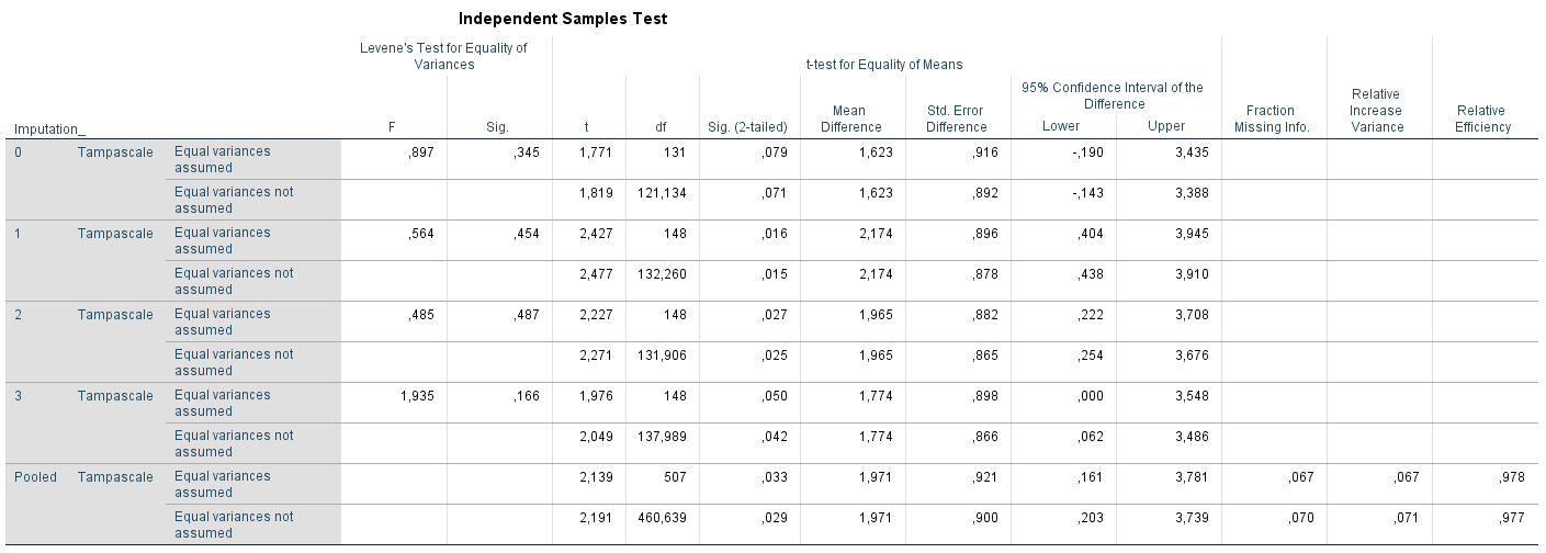
Figure 9.1: T-test for difference in mean Tampascale values between patients with and without Radiation in the leg applied in multiple imputed datasets.
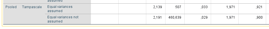
Figure 9.2: T-test for difference in mean Tampascale values between patients with and without Radiation in the leg applied in multiple imputed datasets.
The result in the original dataset (including missing values) is presented in the row that is indicated by Imputation_ number 0. Results in each imputed dataset are shown in the rows starting with number 1 to 3. In the last row which is indicated as “Pooled”, the summary estimates of the mean differences and standard errors are presented. We now explain how these pooled mean differences and standard errors are estimated using RR.
9.1 Pooling Effect estimates
When RR are used, it is assumed that the repeated parameter estimates are normally distributed. This cannot be assumed for all statistical test statistics, e.g. correlation coefficients. For these test statistics, transformations are first performed before RR can be applied.
To calculate the pooled mean differences of Figure 9.1 the following formula is used (9.1):
\[\begin{equation} \bar{\theta} = \frac{1}{m}\left (\sum_{i=1}^m{\theta_i}\right ) \tag{9.1} \end{equation}\]
In this formula, \(\bar{\theta}\) is the pooled parameter estimate, m is the number of imputed datasets, \(\theta_i\) means taking the sum of the parameter estimate (i.e. mean difference) in each imputed dataset i. This formula is equal to the basic formula of taking the mean value of a sequence of numbers.
When we use the values for the mean differences in Figure 9.1, we get the following result for the pooled mean difference:
\[\bar{\theta} = \frac{1}{3}(2.174 + 1.965+1.774)=1.971\]
9.2 Pooling Standard errors
The pooled standard error is derived from different components that reflect the within and between sampling variance of the mean difference in the multiple imputed datasets. The calculation of these components is discussed below.
Within imputation variance This is the average of the mean of the within variance estimate, i.e. squared standard error, in each imputed dataset. This reflects the sampling variance, i.e. the precision of the parameter of interest in each completed dataset. This value will be large in small samples and small in large samples.
\[\begin{equation} V_W = \frac{1}{m} \sum_{i=1}^m{SE_i^2} \tag{9.2} \end{equation}\]
In this formula \(V_W\) is the within imputation variance, m is the number of imputed datasets, \(SE_i^2\) means taking the sum of the squared Standard Error (SE), estimated in each imputed dataset i. Using the standard error estimates in Figure 9.1, we get the following result:
\[V_W = \frac{1}{3}(0.896^2 + 0.882^2 + 0.898^2)=0.7957147\]
Between imputation variance This reflects the extra variance due to the missing data. This is estimated by taking the variance of the parameter of interest estimated over imputed datasets. This formula is equal to the formula for the (sample) variance which is commonly used in statistics. This value is large when the level of missing data is high and smaller when the level of missing data is small.
\[\begin{equation} V_B = \frac{\sum_{i=1}^m (\theta_i - \overline{\theta})^2}{m-1} \tag{9.3} \end{equation}\]
In this formula, \(V_B\) is the between imputation variance, m is the number of imputed datasets, \(\overline{\theta}\) is the pooled estimate, \(\theta_i\) is the parameter estimate in each imputed dataset i.
Using the mean differences in Figure 9.1, we get the following result:
\[V_B = \frac{1}{3-1}((2.174-1.971)^2+ (1.965-1.971)^2+(1.774-1.971)^2)=0.040027\] \[\begin{equation} V_{Total} = V_W + V_B + \frac{V_B}{m} \tag{9.4} \end{equation}\]
\[V_{Total} = 0.7957147+0.040027 + \frac{0.040027}{3}\]
\[SE_{Pooled} = \sqrt{V_{Total}} = \sqrt{0.849084} = 0.9214575\]
This value is equal to the (rounded) pooled standard error value of 0.921 in Figure 9.1.
9.3 Significance testing
For significance testing of the pooled parameter, i.e. the mean difference in Figure 9.1, Formula (9.5) is used. This is the univariate Wald test (Rubin (1987), Van Buuren (2018), Marshall et al. (2009)). This test is defined as:
\[\begin{equation} Wald_{Pooled} =\frac{(\overline{\theta} - {\theta_0})^2}{V_T} \tag{9.5} \end{equation}\]
where \(\overline{\theta}\) is the pooled mean difference and \(V_T\) is the total variance and is equal to the \(SE_{Pooled}\) (pooled standard error) that was derived in the previous paragraph, and \(\theta_0\) is the parameter value under the null hypothesis (which is mostly 0). The univariate Wald test can be used to test all kind of univariate parameters of interest, such as mean differences and univariate regression coefficients from different tpe of regression models. The univariate Wald test in our example is calculated using the pooled regression coefficient and standard error from Figure 9.1:
\[Wald_{Pooled} = \frac{1.971}{\sqrt{0.849084}}=2.139\]
The univariate pooled Wald value follows a t-distribution. This distribution is used to derive the p-value. The value for t depends on the degrees of freedom, according to:
\[\begin{equation} t_{df,1-\alpha/2} \tag{9.6} \end{equation}\]
Where df are the degrees of freedom and \(\alpha\) is the reference level of significance, which is usually set at 5%. The derivation of the degrees of freedom for the t-test is complex. There exist different formula´s to calculate the degrees of freedom and these are explained in the next paragraph.
Because \(t^2\) is equal to F at the same number of degrees of freedom, we can also test for significance using a F-distribution, according to:
\[\begin{equation} F_{1, df}=t^2_{df,1-\alpha/2} \tag{9.7} \end{equation}\]
The degrees of freedom are equal to the degrees of freedom for the t-test above.
9.4 Degrees of Freedom and P-values
The derivation of the degrees of freedom (df) and the p-value for the pooled t-test is not straightforward, because there are different formulas to calculate the df, an older and an adjusted version (Van Buuren (2018)). The older method to calculate the dfs results in a higher value for the df’s for the pooled result than the one in each imputed dataset. An example can be found in Figure 9.3. The degrees of freedoms are 148 in each imputed dataset (in the row for equal variances assumed, under the column df) and 507 for the pooled result. This is important to relize because different values for the df’s lead to different p-values. In SPSS the old way to calculate the dfs is used. Adjusted versions are used in the mice package for R. The differences between the older and adjusted methods to calculate the df’s is illustrated in more detail below.
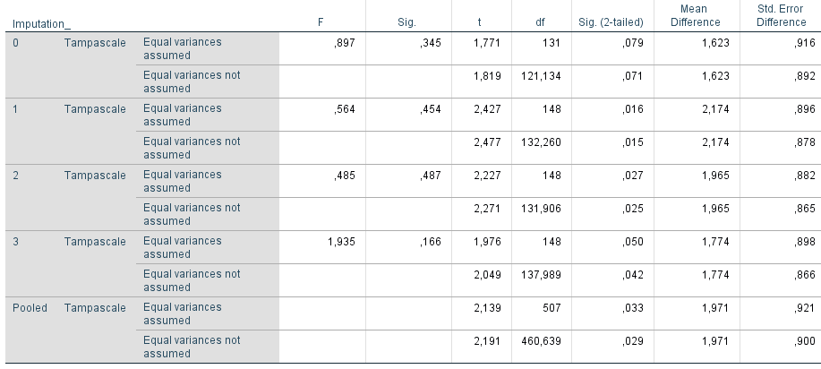
Figure 9.3: Part of Output of Figure 5.1. The value for the dfs are presented in the df column.
The (older method) to calculate the df for the t-distribution is defined as (Rubin (1987), Van Buuren (2018)):
\[\begin{equation} df_{Old} = \frac{m-1}{lambda^2} = (m-1) * (1 + \frac{1}{r})^2 \tag{9.8} \end{equation}\]
Where m is the number of imputed datasets and lambda is equal to the Fraction of Missing information (FMI), calculated by Formula (10.1) (Raghunathan (2016)), and r is the relative increase in variance due to nonresponse (RIV), calculated by Formula (10.2).
The lambda value that is used in Formula (9.8) (and often used as alternative for the FMI) is not the same value for the fraction of missing information of 0.067 that SPSS presents in Figure 9.1. The FMI value of 0.067 is calculated by Formula (10.4) and is called FMI.
When \(df_{old}\) is calculated with the information in Figure 9.3, we get:
\[df_{Old} = \frac{3-1}{0.06283485^2} = 506.5576\]
This (rounded) value is equal to the df value in the row Pooled of 507 in (Figure 9.1). Formula (9.8) leads to a larger df for the pooled result, compared to the dfs in each imputed dataset, which is inappropriate. Therefore, Barnard and Rubin (1999) adjusted this df by using Formula (9.9):
\[\begin{equation} df_{Adjusted} = \frac{df_{Old}*{df_{Observed}}}{df_{Old}+{df_{Observed}}} \tag{9.9} \end{equation}\]
Where \(df_{Old}\) is defined as in Formula (9.8) and \(df_{Observed}\) is defined as:
\[\begin{equation} df_{Observed} = \frac{(n-k)+1}{(n-k)+3}*(n-k)(1-lambda) \tag{9.10} \end{equation}\]
Where n is the sample size in the imputed dataset, k the number of parameters to fit and lambda is obtained by Formula Formula (10.1).
By filling in the formulas (9.10) and (9.9) we get for \(df_{observed}\) and \(df_{adjusted}\) respectively:
\[df_{Observed} = \frac{(150-2)+1}{(150-2)+3}*(150-2)(1- 0.06283485)=136.8633\]
\[df_{Adjusted} = \frac{(506.5576* 136.8633)}{(506.5576+ 136.8633)}=107.7509\]
The number of 107.7509 is equal to the df used by mice.
We can now derive the p-value for the pooled mean difference in the Tampascale between patients with and without Radiation in the leg. This two-sided p-value is:
In SPSS:
\[t_{df,1-\alpha/2}=2.139_{df{Old}}=0.03289185\]
In R:
\[t_{df,1-\alpha/2}=2.139_{df{Adjusted}}=0.03467225\]
9.5 Confidence Intervals
For the 95% confidence interval (CI), the general formula can be used:
\[\begin{equation} \bar{\theta} ± t_{df,1-\alpha/2} * SE_{Pooled} \tag{9.11} \end{equation}\]
In this formula, \(\bar{\theta}\) is the pooled estimate, t is the t-statistic, df is degrees of freedom and \(SE_{Pooled}\) is the pooled standard error (Formula (9.4)).