Chapter4 Multiple Imputation
In this Chapter we discuss an advanced missing data handling method, Multiple Imputation (MI). With MI, each missing value is replaced by several different values and consequently several different completed datasets are generated. The concept of MI can be made clear by the following figure 4.1.
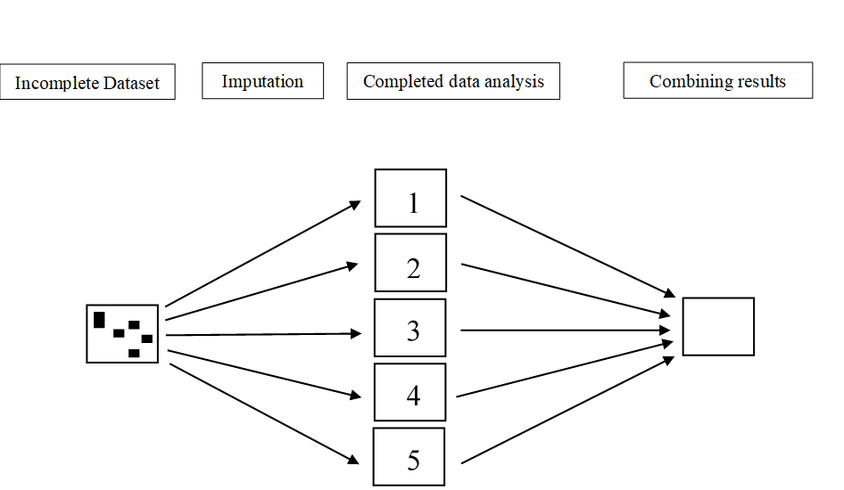
Figure 4.1: Graphical presentation of the MI procedure.
In the first step, the dataset with missing values (i.e. the incomplete dataset) is copied several times. Then in the next step, the missing values are replaced with imputed values in each copy of the dataset. In each copy, slightly different values are imputed due to random variation. This results in mulitple imputed datasets. In the third step, the imputed datasets are each analyzed and the study results are then pooled into the final study result. In this Chapter, the first phase in multiple imputation, the imputation step, is the main topic. In the next Chapter, the analysis and pooling phases are discussed.
4.1 Multivariate imputation by chained equations (MICE)
Multivariate imputation by chained equations (MICE) (Van Buuren 2018) is also known as Sequential Regression Imputation, Fully Conditional Specification or Gibbs sampling. In the MICE algorithm, a chain of regression equations is used to obtain imputations, which means that variables with missing data are imputed one by one. The regression models use information from all other variables in the model, i.e. (conditional) imputation models. In order to add sampling variability to the imputations, residual error is added to create the imputed values. This residual error can either be added to the prediced values directly, which is esentially similar to repeating stochastic regression imputation over several imputation runs. Residual variance can also be added to the parameter estimates of the regression model, i.e. the regression coefficients, which makes it a Bayesian method. The Bayesian method is the default in the mice package in R. The MICE procedure became available in SPSS when version 17 was released.
4.2 Multiple imputation in SPSS
We use as an example a dataset with 50 patient with low back pain. In these patients information was measured about their Pain, Tampa scale, Disability and Radiation. The variables Tampa scale and Disability contain missing values of 26% and 18% respectively.
The multiple imputation procedure is started by navigating to
Analyze -> Multiple Imputation -> Impute Missing Data Values.
Than a window opens that consists of 4 tabs, a Variables, a Method, a Constraints and an Output tab. You have to visit these tabs to specify the imputation settings before you can start the imputation process by clicking the OK button.
4.2.1 The Variables tab
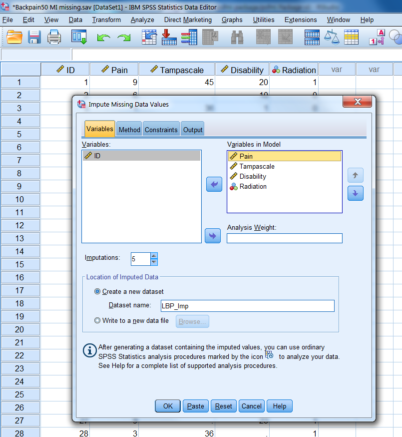
Figure 4.2: The variables Tab
The first window is the Variables tab (Figure 4.2). Here you can transport the complete and incomplete variables that you want to include in the imputation model to the window “Variables in Model”. The variables are imputed sequentially in the order in which they are listed in the variables list. These variables are here Pain, Tampa scale, Disability and Radiation. In our example the Tampa scale variable is imputed before the Disability variable because the Tampa scale variable was first listed. Further, the number of imputed datasets can be defined in the “Imputations”” box, we choose 5 here. Than you go to “Create a new Dataset” and choose a name for the dataset to which the imputed data values are saved, which is called “LBP_Imp”. If you are finished you visit the Methods Tab where you can define the imputation method.
4.2.2 The Method tab
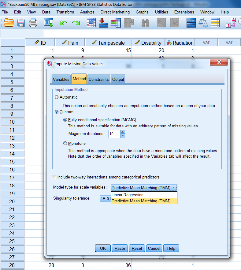
Figure 4.3: The Methods Tab
In the Method tab (Figure 4.3) you choose the imputation algorithm. We choose for “Custom” under Imputation Method and for Fully conditional specification (FCS). FCS is the Bayesian regression imputation method as explained in Chapter 3. You can also change the maximum number of Iterations which has a default setting of 10. It is recommended to increase that number to 50. Under Model type for scale (continuous) variables we choose for Predictive Mean Matching (PMM) (see paragraph 4.6 for a more detailed explanation of PMM). PMM is the default procedure in the mice package to impute continuous variables. In SPSS the default is the linear regression procedure. It is better to change it into PMM. Now visit the Constraints Tab.
4.2.3 The Constraints tab
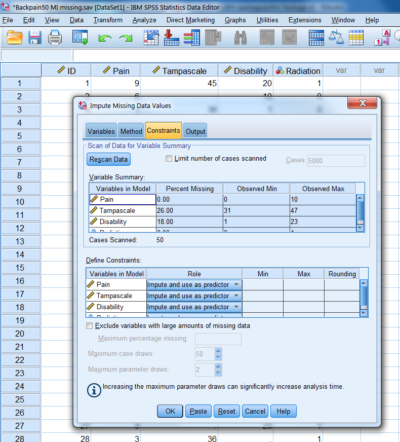
Figure 4.4: The Constraints Tab
In the Constraints tab (Figure 4.4) the minimum and maximum allowable imputed values for continuous variables can be defined when for scale variables the Linear Regression model is chosen in the Method tab. To obtain the current range of variable values you can click on the “Scan” button, subseqeuntly these values can be adjusted. When the PMM method is selected in the Method Tab, the Constraints tab can be skipped. You can also restrict the analysis to variables with less than a maximum percentage of missing values when you select “Exclude variables with large amounts of missing data”. In the Constraints tab also the role of variables in the imputation model can be defined (see paragraph 4.2.5). In the last Output Tab the generated output can be selected.
4.2.4 The Output tab
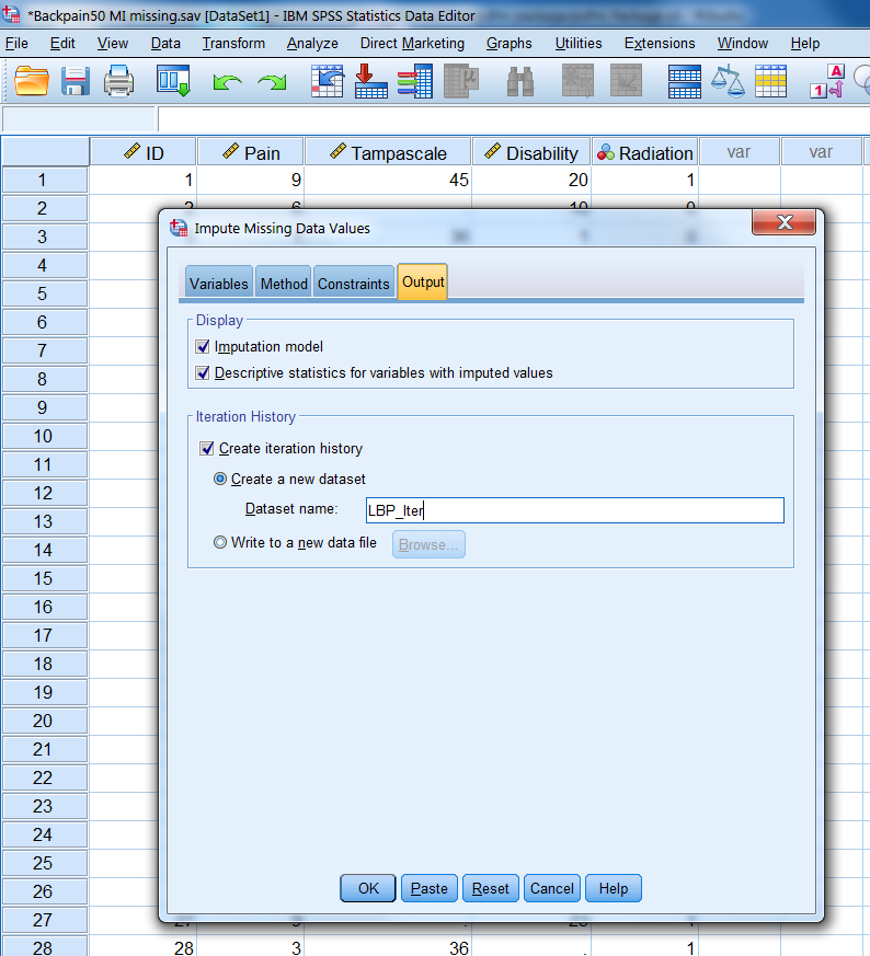
Figure 4.5: The Output Tab
In the Output tab (Figure 4.5) descriptive statistics of variables that are imputed can be exctracted by selecting “Imputation model” and “the Descriptive statistics for variables with imputed values” options. You can also request a dataset that contains iteration history data, which we name “Iter_Backpain”. The dataset contains the means and standard deviations of the imputed scale variables at each iteration. You can use this data to check for irregularities during imputation by making convergence plot that will be discussed in paragraph 4.5.
4.2.5 Customizing the Imputation Model
The content of the imputation model, i.e. regression model used to impute missing values, is important to generate valid imputed values. The role of variables in the imputation model before MI is started can be customized in SPSS in the Constraints tab. As default all variables that are transported to the window “Variables in Model” in the first Variables tab will be imputed or used as a predictor in the imputation model by using the default setting “Impute and use as predictor”. This setting means that any variable is used as a predictor in the imputation model to predict missing values in any other variable. This role of variables can be adjusted in the Constraints tab by using a variable as a predictor only, by the setting “Use as predictor only” or to exclude variables from being used as predictors in the imputation model by the setting “Impute only” for example for variables with larger percentages of missing data. Note that when in SPSS a variable is used as a predictor to impute variables with missing data, that variable will be part of each imputation model to impute every other variable with missing data. This may lead to large imputation models that may contain variables that are not the best predictors to impute missing values when their correlation with other variables is low.
4.3 Random number generator
Before you start the multiple imputation procedure, it is possible to set the starting point of the random number generator in SPSS at a fixed value of 950 (in R we use the seed for this). In this way you are able to reproduce results exactly. later. It is also a good idea to store the multiple imputed datasets.
We set the random number generator in SPSS via
Transform -> Random Number Generators -> Set Starting point -> Fixed Value
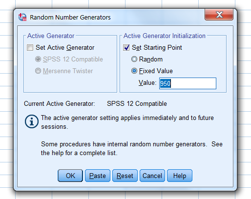
Figure 4.6: Set the Random Number Generator
4.4 The output of Multiple imputation in SPSS
4.4.1 The Imputed datasets
After multiple imputation, the multiple imputed datasets are stored in a new SPSS file and are stacked on top of each other. A new variable that is called Imputation_ is added to the dataset and can be found in the first column. This Imputation_ variable is a nominal variable that separates the original from the imputed datasets. This is also indicated in the corner on the right side below in the Data View and Variable View windows by the note “Split by imputation_”. You can compare the use of this variable with the Split File option in SPSS where all analyses are done separately for the categories of the variable used to split the analyses. The difference is that with the Imputation_ variable you also obtain pooled estimates for the statistical analyses. When missing values are imputed with any another software program, and you read in the imputed data in SPSS and add an Imputation_ variable yourself the data is recognized by SPSS as multiple imputed data. The imputed values are marked yellow. By these marking SPSS recognized the dataset as an (multiple) imputed dataset which is important for further statistical analyses (see Chapter 5, paragraph 5.1)
Figure 4.7 shows an example of a multiple imputed dataset with imputed values marked yellow.
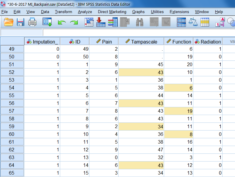
Figure 4.7: Example of SPSS dataset after MI has been applied.
You can mark and unmark the imputed values by using the option “Mark Imputed Data” under the View menu in the Data View window (Figure 4.8).
View -> Mark Imputed data
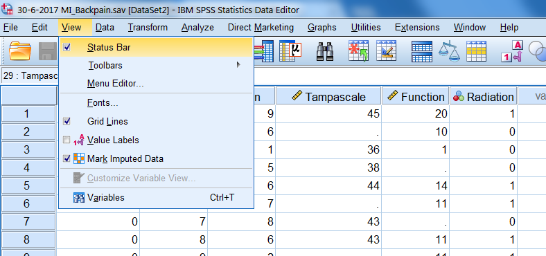
Figure 4.8: Procedure to mark imputed values in SPSS.
This marking and unmarking can also be done in the Data view window via the button with yellow and white squares on the right site above (Figure 4.9). If you click the button, a selection box appears with “Original data” selected,where you can easily move to the different imputed datasets.
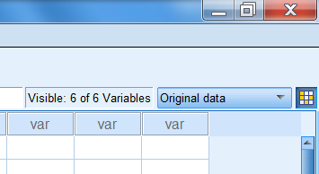
Figure 4.9: Button and selection box to mark imputed values
4.4.2 Imputation history
The iteration history is stored in the Iter_Backpain dataset as we defined in the Output window. In this dataset the means and standard deviations of the imputed values at each iteration are stored. These values can be used to construct Convergence plots. More about making convergence plots will be discussed in the next paragraph.
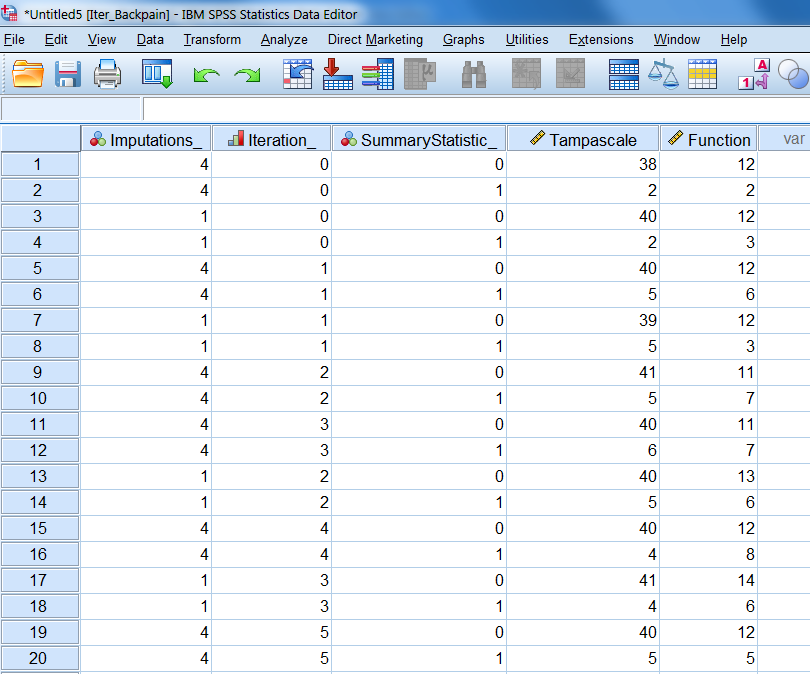
Figure 4.10: The iteration history data
4.4.3 Output tables
Based on our settings, SPSS produces the following results in the output window. In the Imputation Specifications table, information is provided on the imputation method used, the number of imputations, the model used for the scale variables, if interactions were included in the imputation models, the setting for the maximum percentage of missing values and the setting for the maximum number of parameters in the imputation model (Figure 4.11).
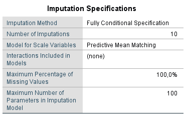
Figure 4.11: Imputation Specifications table
A second table, called Imputation Results, is presented with information about the imputation method, the number of fully conditional specification methods, the variables that are imputed and not imputed and the imputation sequence(Figure 4.12).
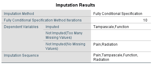
Figure 4.12: Imputation Results
The Imputation Models table presents information about the imputation models used for the variables with missing data (Figure 4.13). Information is provided about the method of imputation, under the type column, the effect estimates used to impute the missing values, the number of missing and imputed values. For example for the Tampascale variable 13 values were missing and m=5 times 13 is 65 values were imputed.
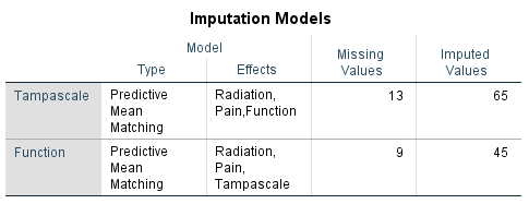
Figure 4.13: Imputation Models
The Descriptive statistics display the descriptive information of the original, imputed and completed data of the Tampascale and the Disability variable. In this way you can compare the completed data after MI with the original data.
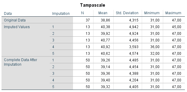
Figure 4.14: Descriptive statistics
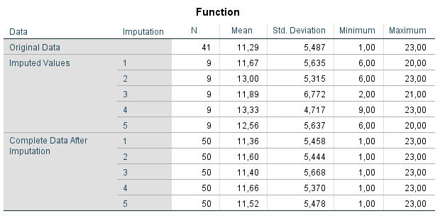
Figure 4.15: Descriptive statistics
4.5 Checking Convergence in SPSS
The dataset Iter_Backpain in the previous paragraph contains the means and standard deviations of the imputed values at each iteration and imputation round. This information is similar as the
information in imp$chainMean in R. This dataset can be used to generate convergence plots, to check if the imputed values have the expected variation between the iterations.The iteration can be checked for the means and standard deviations seperately. In order to obtain seperate plots for these summary statistics, the split file option in SPSS can be activated.
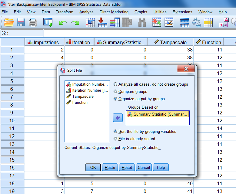
Figure 4.16: Split file
After activation of the split file option, the Graph menu in SPSS can be used to make the plots.
Graph -> Chart Builder.
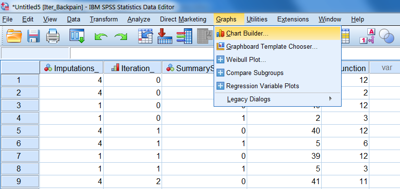
Figure 4.17: Graph menu
Two windows will open that can be used to build a chart:
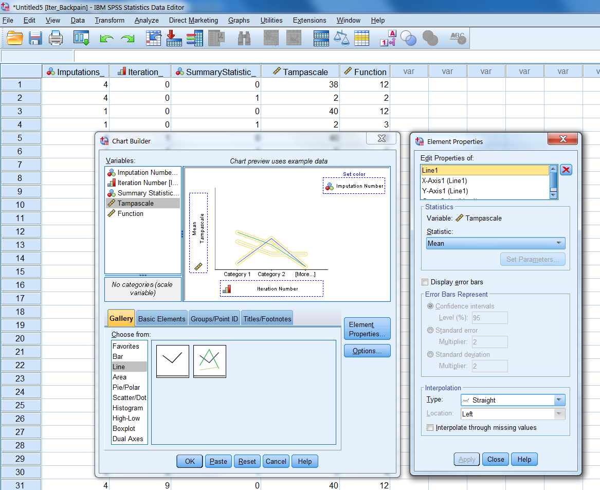
Figure 4.18: Chart Builder
On the x-axis the put the iteration number variable and on the y-axis the variable for which we want to display the iteration history. The Imputation Number variable is dragged to the set color top-right.
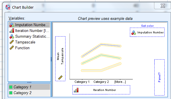
Figure 4.19: Chart Builder
As a result two plots appear with the iteation history for each imputation run.
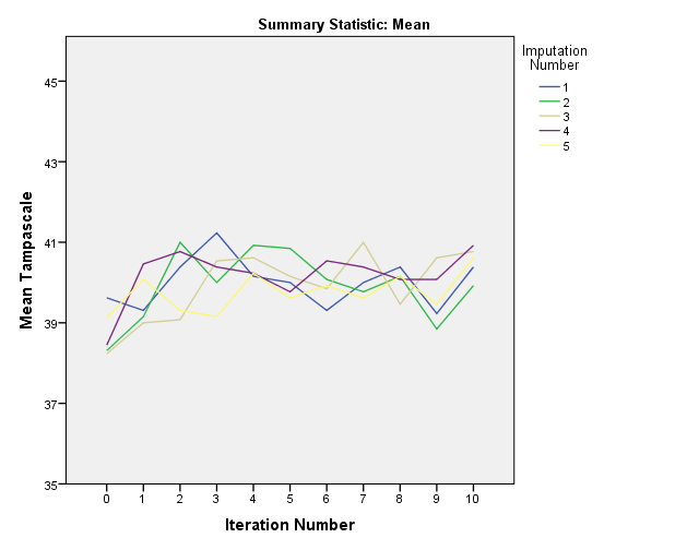
Figure 4.20: Convergence plots
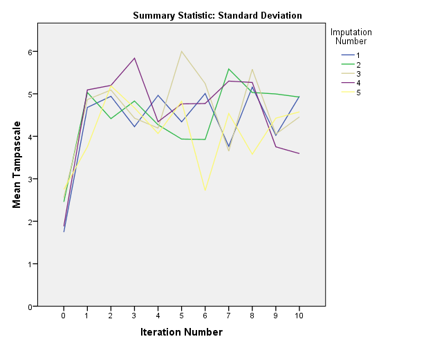
Figure 4.21: Convergence plots
4.6 Multiple Imputation in R
In R multiple imputation (MI) can be performed with the mice function from the mice package. As an example dataset to show how to apply MI in R we use the same dataset as in the previous paragraph that included 50 patients with low back pain. The variables Tampa scale and Disability contain missing values and the Pain and Radiation variables are complete.
The following default settings are used in the mice function to start MI, m=5, to generate 5 imputed datasets, maxit=10, to use 10 iterations for each imputed dataset, method=”pmm” to use predictive mean matching (see paragraph 4.11). For an elobate explanation of all options withing the mice function, see ?mice.
library(mice)
library(foreign)
data <- read.spss(file="data/Backpain50 MI missing.sav", to.data.frame=T)[, -1] # Read in dataset an exclude ID variable
imp <- mice(data, m=5, maxit=10, method="pmm")
##
## iter imp variable
## 1 1 Tampascale Disability
## 1 2 Tampascale Disability
## 1 3 Tampascale Disability
## 1 4 Tampascale Disability
## 1 5 Tampascale Disability
## 2 1 Tampascale Disability
## 2 2 Tampascale Disability
## 2 3 Tampascale Disability
## 2 4 Tampascale Disability
## 2 5 Tampascale Disability
## 3 1 Tampascale Disability
## 3 2 Tampascale Disability
## 3 3 Tampascale Disability
## 3 4 Tampascale Disability
## 3 5 Tampascale Disability
## 4 1 Tampascale Disability
## 4 2 Tampascale Disability
## 4 3 Tampascale Disability
## 4 4 Tampascale Disability
## 4 5 Tampascale Disability
## 5 1 Tampascale Disability
## 5 2 Tampascale Disability
## 5 3 Tampascale Disability
## 5 4 Tampascale Disability
## 5 5 Tampascale Disability
## 6 1 Tampascale Disability
## 6 2 Tampascale Disability
## 6 3 Tampascale Disability
## 6 4 Tampascale Disability
## 6 5 Tampascale Disability
## 7 1 Tampascale Disability
## 7 2 Tampascale Disability
## 7 3 Tampascale Disability
## 7 4 Tampascale Disability
## 7 5 Tampascale Disability
## 8 1 Tampascale Disability
## 8 2 Tampascale Disability
## 8 3 Tampascale Disability
## 8 4 Tampascale Disability
## 8 5 Tampascale Disability
## 9 1 Tampascale Disability
## 9 2 Tampascale Disability
## 9 3 Tampascale Disability
## 9 4 Tampascale Disability
## 9 5 Tampascale Disability
## 10 1 Tampascale Disability
## 10 2 Tampascale Disability
## 10 3 Tampascale Disability
## 10 4 Tampascale Disability
## 10 5 Tampascale DisabilityBy default, the mice fucntion returns information about the iteration and imputation steps of the imputed variables under the columns named “iter”, “imp” and “variable” respectively. This information can be turned off by setting the mice function parameter printFlag = FALSE, which results in silent computation of the missing values. A summary of the imputation results can be obtained by calling the imp object.
imp## Class: mids
## Number of multiple imputations: 5
## Imputation methods:
## Pain Tampascale Disability Radiation
## "" "pmm" "pmm" ""
## PredictorMatrix:
## Pain Tampascale Disability Radiation
## Pain 0 1 1 1
## Tampascale 1 0 1 1
## Disability 1 1 0 1
## Radiation 1 1 1 0This imp object returns information about the number of imputed datasets, the imputation methods for each variable, information of the PredictorMatrix (used to customize the imputation model, see paragraph 4.6.2).
The imputed datasets can be extracted by using the complete function. The settings action = ”long” and include = TRUE returns a dataframe where the imputed datasets are stacked under each other and the original dataset (with missings) is included on top.
complete(imp, action = "long", include = TRUE)In the imputed datasets two variables are added, an .id variable and an .imp variable to distinguish cases and the imputed datasets. To extract the first imputed dataset, only the setting action = 1 is needed in the complete function. (see ?complete for more possibilities to extract the imputed datasets).The imputed datasets can further be used in mice to conduct pooled analyses or to store them for further use.
4.7 Setting the imputation methods
The default imputation methods for continous, dichotomous and categorical variables in the mice function are pmm, logreg and polyreg respectively. For complete variables without missing data the default method is set as "".
For example, we assume that we have missing data in two continuous and one dichotomous variable, i.e. the Tampa scale, Disability and Radiation variables. After we have multiple imputed the missing values we can extract the imputation method for each variable by running:
library(mice)
library(haven)
# Read in dataset an exclude ID variable
data <- read_sav(file="data/Backpain50 MI missing all.sav")[, -1]
data$Radiation <- factor(data$Radiation)
imp <- mice(data, m=5, maxit=10, printFlag = FALSE)
imp$method
## Pain Tampascale Disability Radiation
## "" "pmm" "pmm" "logreg"If we want to change the imputation method for the Tampa scale variable from "pmm" into "norm" (Bayesian linear regression without predictive mean matching) we first run:
impmethod <- imp$method
impmethod["Tampascale"] <- "norm"
impmethod## Pain Tampascale Disability Radiation
## "" "norm" "pmm" "logreg"The adjusted method can subsequently be used in the mice function:
imp <- mice(data, m=5, maxit=10, method = impmethod, printFlag = FALSE)You can also change the imputation method before you do a full multiple imputation analysis by running mice first using the settings m=1 and maxit=0. Subsequently, you can adjust the imputation method for specific variables and run the full multiple imputation procedure, using the new imputation method.
4.8 The MI Shiny app
During the imputation process the mice fucntion returns information about the iteration and imputation steps of the imputed variables under the columns named “iter”, “imp” and “variable” respectively. During this process missing values are filled in by using a chain of regression models. This is a rather complicated process. To get some more insight in what happens during the interation and imputation steps we shortly describe the imputation of the missing values in the Tampa scale and Disability variables during the first two iteration steps below.
We have also developed a Shiny app to explain MI in more detail. This is an interactive learning app of how MI with mice works and shows how the imputed values in the Tampa scale and Disability variables are calculated. Click on Shiny app to use the app.
Iteration 0 Per imputed dataset at iteration number 0 values are randomly drawn from the observed values of the Tampa scale and Disability variable and these are used to replace the missing values in these variables.
Iteration 1 At this step the Tampa scale values are set back to missing. Subsequently, a linear regression model is applied in the available data (i.e. all subjects with observed Tampa scale values) using the Tampa scale as the dependent variable and the Pain, Disability and Radiation variables as independent variables. From this regression model the missing Tampa scale values are imputed. Note that for this regression model the imputed values for the Disability variable are used from the previous iteration step of 0. The Baysian stochastic regression imputation method adds uncertainty to the imputed values via the error variance (residuals) and the regression coefficients. This regression model is defined as:
\(Tampa_{mis} = \beta_0 + \beta_1Pain + \beta_2Disability + \beta_3Radiation\)
The same procedure is repeated for the Disability variable. The Disability scores are first set back to missing, then the regression coefficients for the Pain, Tampa scale and Radiation variables are obtained from the subjects without missing Disability values. Note that now the imputed values for the Tampa scale variable. The imputed values for Disability are estimated using (Bayesian) regression coefficients with additional error variance to the residuals. This regression model is defined as:
\(Disability_{mis} = \beta_0 + \beta_1Pain + \beta_2Tampa + \beta_3Radiation\)
Iteration 2 For iteration 2 the Tampa scale values are again set back to missing and (new) updated regression coefficients for Pain, Disability and Radiation are obtained, using the imputed values for Disability from iteration 1. Accordingly, missing values are estimated from the regression model, again using Bayesian regression coefficients. The same holds for the Disability variable. The imputed values for the Disability variable are estimated from the regression model using the imputed values in the Tampa scale variable within the same iteration number.
This process is repeated in each following iteration until the final iteration where the imputed values are used for the first imputed dataset. For the next imputed dataset, the entire process of iterations is repeated.
4.9 Customizing the Imputation model
During MI in the example of paragraph 4.6 above the variables Tampa scale and Disability were imputed with the help of the variables Pain and Radiation. The latter two variables are called auxiliary variables when they are not part of the main analysis model but they help to impute the Tampa scale and Disability variables. These variables are included in the imputation model to impute the missing data in the Tampa scale and Disability variables.
To define the imputation model for variables with missing data mice makes use of a predictor matrix. The predictor matrix is a matrix with the names of the variables in the dataset listed in the rows and the columns. The variables in the columns are used to impute the row variables. They are part of the imputation model. As a default setting all variables that are included in the dataset are used as predictors to impute missing values. The predictor matrix that is used in the mice function can be obtained by typing:
library(mice)
library(foreign)
data <- read.spss(file="data/Backpain50 MI missing.sav", to.data.frame=T)[, -1] # Read in dataset an exclude ID variable
imp <- mice(data, m=5, maxit=10, method="pmm", printFlag = FALSE)imp$predictorMatrix## Pain Tampascale Disability Radiation
## Pain 0 1 1 1
## Tampascale 1 0 1 1
## Disability 1 1 0 1
## Radiation 1 1 1 0Variables in the columns can be switched on or off by using a 1 or a 0 to in- or exclude them from the imputation model. In this way the imputation models for each variable with missing data can be customized. For example, the variable in the second row, i.e. the Tampa scale variable, contains missing values and the 1´s in this row mean that the column variables Pain, Disability and Radiation are included in the imputation model to impute the Tampa scale variable. For the Disability variable, the variables Pain, Tampa scale and Radiation are used.
The predictor matrix can be adapted when for example a variable that contains a high percentage of missing data should be excluded from the imputation model. If we want to exclude the variable Disability from the imputation model of the Tampa scale variable we can change the value of 1 for the Disability variable into 0.
pred <-imp$predictorMatrix
pred["Tampascale", "Disability"] <- 0
pred## Pain Tampascale Disability Radiation
## Pain 0 1 1 1
## Tampascale 1 0 0 1
## Disability 1 1 0 1
## Radiation 1 1 1 0This adjusted predictor matrix could than be re-used in the mice function by refrerring to it.
imp <- mice(data,m=5, maxit=10, method="pmm", predictorMatrix = pred)The diagonal of the predictor matrix always contains zeroes, because variables cannot be included in their own imputation model.
4.10 Guidelines for the Imputation model
There are several guidelines that can be used to customize the imputation model for each variable by the predictor matrix (Collins, Schafer, and Kam (2001), Van Buuren (2018), Rubin (1976)). To summarize:
- Include all variables that are part of the analysis model, including the dependent (outcome) variable.
- Include the variables at the same way in the imputation model as they appear in the analysis model (i.e. if interaction terms are in the analysis model also include them in the imputation model).
- Include additional (auxiliary) variables that are related to missingness or to variables with missing values.
- Be aware of including variables with a high correlation (> 0.90).
- Be aware of variables with high percentages of missing data (> 50%).
4.11 Output of the mice function
The mice function returns a mids (multiple imputed data set) object. In this object, imputation information is stored and can be extracted by typing imp$, followed by the type of information you want to obtain.
imp$m
imp$nmis
imp$seed
imp$iterationThe above objects contain the the number of imputed datasets, missing values in each variable, the specified seed value (NA here because we did not define one) and the number of iterations.
The original data can be found in:
imp$dataThe imputed values for each variable in the imptued values can be found under:
imp$impThe imputation methods used:
imp$methodThe predictor matrix:
imp$predictorMatrixThe sequence of the variables used in the impution procedure:
imp$visitSequence4.11.1 Checking Convergence in R
The convergence of the imputation procedure can be evaluated. The means of the imputed values for each iteration can be extracted as chainMean.
imp$chainMean## , , Chain 1
##
## 1 2 3 4 5 6 7
## Pain NaN NaN NaN NaN NaN NaN NaN
## Tampascale 40.84615 39.15385 41.53846 40.61538 42.15385 40.46154 40.00000
## Disability 13.00000 10.22222 12.66667 10.77778 12.00000 12.00000 12.66667
## Radiation NaN NaN NaN NaN NaN NaN NaN
## 8 9 10
## Pain NaN NaN NaN
## Tampascale 40.76923 40.15385 41.30769
## Disability 10.11111 12.22222 10.00000
## Radiation NaN NaN NaN
##
## , , Chain 2
##
## 1 2 3 4 5 6 7
## Pain NaN NaN NaN NaN NaN NaN NaN
## Tampascale 40.15385 41.23077 39.84615 40.30769 40.84615 40.15385 39.69231
## Disability 11.33333 11.88889 11.11111 10.66667 12.88889 12.11111 14.55556
## Radiation NaN NaN NaN NaN NaN NaN NaN
## 8 9 10
## Pain NaN NaN NaN
## Tampascale 40.76923 39.92308 39.92308
## Disability 12.66667 11.66667 11.44444
## Radiation NaN NaN NaN
##
## , , Chain 3
##
## 1 2 3 4 5 6 7
## Pain NaN NaN NaN NaN NaN NaN NaN
## Tampascale 39.69231 41.15385 41.07692 40.46154 40.84615 40.46154 40.76923
## Disability 11.33333 12.44444 11.44444 10.55556 10.33333 12.77778 12.88889
## Radiation NaN NaN NaN NaN NaN NaN NaN
## 8 9 10
## Pain NaN NaN NaN
## Tampascale 41.61538 39.84615 39.23077
## Disability 10.55556 11.88889 11.33333
## Radiation NaN NaN NaN
##
## , , Chain 4
##
## 1 2 3 4 5 6 7
## Pain NaN NaN NaN NaN NaN NaN NaN
## Tampascale 40.00000 38.92308 40.53846 40.15385 40.00000 40.23077 41.076923
## Disability 10.77778 10.44444 12.77778 12.77778 11.88889 10.77778 9.666667
## Radiation NaN NaN NaN NaN NaN NaN NaN
## 8 9 10
## Pain NaN NaN NaN
## Tampascale 40.30769 39.53846 41.46154
## Disability 10.11111 14.00000 10.11111
## Radiation NaN NaN NaN
##
## , , Chain 5
##
## 1 2 3 4 5 6 7
## Pain NaN NaN NaN NaN NaN NaN NaN
## Tampascale 40.76923 40.07692 39.76923 39.84615 40.30769 41.30769 40.53846
## Disability 12.33333 10.33333 11.66667 12.00000 10.66667 11.44444 14.00000
## Radiation NaN NaN NaN NaN NaN NaN NaN
## 8 9 10
## Pain NaN NaN NaN
## Tampascale 40.84615 39.00000 40.15385
## Disability 12.00000 11.66667 12.66667
## Radiation NaN NaN NaNThe number of chains is equal to the number of imputed datasets. A chain refers to the chain of regression models that is used to generate the imputed values. The length of each chain is equal to the number of iterations.
The convergence can be visualised by plotting the means in a convergence plot. For our example, the convergence plots are shown below. In this plot you see that the variance between the imputation chains is almost equal to the variance within the chains, which indicates healthy convergence.
plot(imp)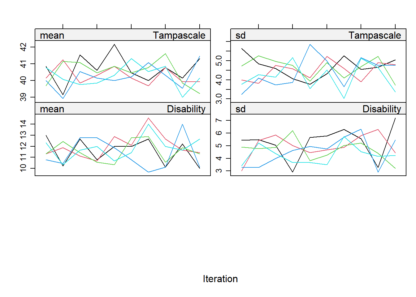
4.11.2 Imputation diagnostics in R
It can also be of interest to compare the values that are imputed with those that are observed. For that, the stripplot function can be used in mice. This function visualises the observed and imputed values in one plot. By comparing the observed and the imputed data points we get an idea if the imputed values are in range of the observed data. If there are no large differences between the imputed and observed values than we can conclude the imputed values are plausible.
stripplot(imp)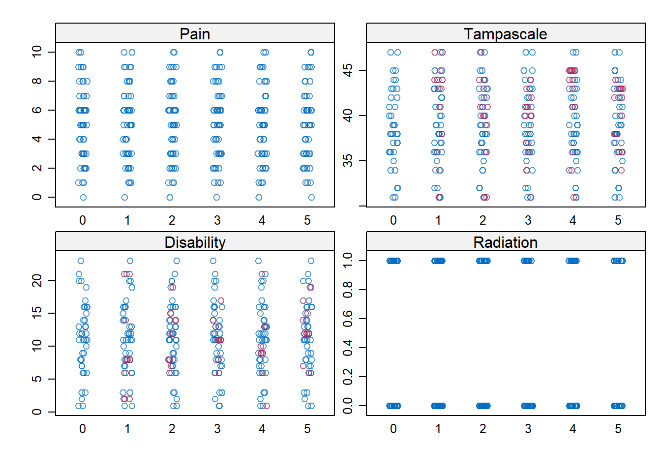
4.12 Predictive Mean Matching or Regression imputation
Within the mice algorithm continuous variables can be imputed by two methods, linear regression imputation or Predictive Mean Matching (PMM). PMM is an imputation method that predicts values and subsequently selects observed values to be used to replace the missing values. We recommend to use PMM during imputation. It is the default imputation procedure in the mice package (Rubin 1987). In SPSS the default imputation procedure is linear regression.
4.12.1 Predictive Mean Matching, how does it work?
The Predictive Mean Matching algorithm takes place in several steps:
We take as an example a dataset with 10 cases with 3 missing values in the Tampa scale variable. They are defined as NA in the dataset below. The Pain variable is used to predict the missing Tampa scale values.
## ID Pain Tampascale
## 1 1 5 40
## 2 2 6 NA
## 3 3 1 41
## 4 4 5 42
## 5 5 6 44
## 6 6 7 NA
## 7 7 8 43
## 8 8 6 40
## 9 9 2 NA
## 10 10 6 38Step 1: Estimate a linear regression model
A linear regression model is estimated with the Tampa scale variable as the outcome and the Pain variable as the predictor variable. We define the regression coefficient for Pain as \(\hat{\beta_{Pain}}\).
Step 2: Determine Bayesion version of regression coefficient
A Bayesian regression coefficient for the Pain variable is determined. We define this regression coefficient as \(\beta_{Pain}^*\).
Step 3: Predict Missing values
Observed Tampa scale valueas are predicted by the Pain regression coefficient \(\hat{\beta_{Pain}}\) from step 1 and the Pain data, we call these values \(Tampa_{Obs}\) and can be found in the Table below.
Missing Tampa scale valueas are predicted by the regression coefficient \(\beta_{Pain}^*\) from step 2 and the Pain data, we call these \(Tampa_{Pred}\).
These values for the three missing Tampa scale are: 43.594, 41.456 and 39.852.
Step 4: Find closest donor
Find the closest donor for the first missing value by subtracting the first \(Tampa_{Pred}\) value of 43.594 from all predicted observed values in the \(Tampa_{Obs}\) column. These differences are shown in the column Difference in the table below.
| ID | Pain | Tampascale | Tampa_Obs | Difference |
|---|---|---|---|---|
| 1 | 5 | 40 | 42.020 | 1.574 |
| 2 | 6 | NA | NA | NA |
| 3 | 1 | 41 | 41.624 | 1.970 |
| 4 | 5 | 42 | 41.426 | 2.168 |
| 5 | 6 | 44 | 41.228 | 2.366 |
| 6 | 7 | NA | NA | NA |
| 7 | 8 | 43 | 40.832 | 2.762 |
| 8 | 6 | 40 | 40.634 | 2.960 |
| 9 | 2 | NA | NA | NA |
| 10 | 6 | 38 | 40.238 | 3.356 |
The smallest differences are 1.574, 1.970 and 2.168 and these belong to the cases with observed Tampa scale values of 40, 41 and 42 respectively. Subsequently, a value is randomly drawn from these observed values and used to impute the first missing Tampa scale value. Other missing values are imputed by following the same procedure, i.e. now subtracting the second \(Tampa_{Pred}\) value of 41.456 from all predicted observed alues and finding the closest match.
The strength of PMM is that missing data is replaced by data that is observed in the dataset and not replaced by unrealistic values (as negative Tampa scale scores). PMM can therefore handle better the imputation of variables with skewed distributions or non-linear relationships between variables.
4.13 Imputation of categorical variables
The mice procedure in SPSS and R uses for the imputation of continuous variables linear regression models, for dichotomous variables, logistic regression models and for categorical variables with >2 categories polytomous regression models. To be sure that the correct regression model is used it is important to define the level of measurement of the variable with missing data before MI is started. In SPSS this is possible in the Variable View window where variables can be defined as scale, nominal or ordinal. In R categorical variables can be defined as categorical in the Console window, or in the script file by using the function factor.
If categorical variables are not defined as categorical, linear regression models will be used to impute them because they are used as default method in SPSS and R (via the default method pmm). Instead of discrete values that represent the different categories, continuous values will be imputed. Figure 4.22 shows what happens when the dichtomous variable Radiation is defined as a scale variable and MI is applied in SPSS using the default method Linear Regression. The imputed values are estimated by using linear regression models and even negative values are used to replace missing values. This error could be solved by choosing predictive mean matching (PMM) as imputation method, than 0’s and 1’s will be imputed. However still linear regression models would be used as basic method to generate predicted values. Changing the measurement level of the variable from scale to nominal is the best choice.
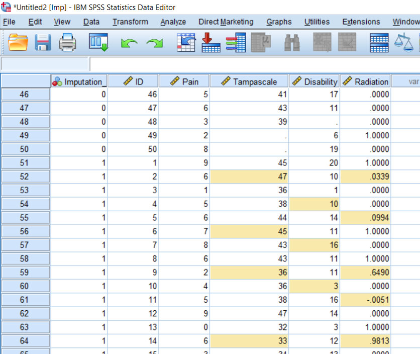
Figure 4.22: Incorrect Imputation of the variable Radiation
Coding of the level of the variable Radiation from continous to categorical is also needed in R. Even if you define the variable as being a nominal variable in SPSS before you read that data in into R, R still assumes that it is a continuous variable and uses PMM and thus linear regression models as imputation method. This can be corrected by using the function
factor in R before you run MI.
Incorrect imputation
library(mice)
library(foreign)
# Read in dataset an exclude ID variable
data <- read.spss(file="data/Backpain50 MI missing radiation.sav", to.data.frame=T)[, -1]
imp <- mice(data, m=5, maxit=10, printFlag = FALSE)
imp## Class: mids
## Number of multiple imputations: 5
## Imputation methods:
## Pain Tampascale Disability Radiation
## "" "pmm" "pmm" "pmm"
## PredictorMatrix:
## Pain Tampascale Disability Radiation
## Pain 0 1 1 1
## Tampascale 1 0 1 1
## Disability 1 1 0 1
## Radiation 1 1 1 0Correct Imputation
See the correct imputation method logreg for the variable Radiation.
library(mice)
library(foreign)
# Read in dataset an exclude ID variable
data <- read.spss(file="data/Backpain50 MI missing radiation.sav", to.data.frame=T)[, -1]
data$Radiation <- factor(data$Radiation)
imp <- mice(data, m=5, maxit=10, printFlag = FALSE)
imp## Class: mids
## Number of multiple imputations: 5
## Imputation methods:
##       Pain Tampascale Disability  Radiation
##         ""      "pmm"      "pmm"   "logreg"
## PredictorMatrix:
##            Pain Tampascale Disability Radiation
## Pain          0          1          1         1
## Tampascale    1          0          1         1
## Disability    1          1          0         1
## Radiation 1 1 1 0It seems that you can not completely solve the problem by using logreg as imputation method in the mice function before you run MI because than the following message appears in the Console window Type mismatch for variable(s): Radiation Imputation method logreg is for categorical data. This message will disappear after you have defined the variable Radiation as a categorical variable with the function factor.
library(mice)
library(foreign)
# Read in dataset an exclude ID variable
data <- read.spss(file="data/Backpain50 MI missing radiation.sav", to.data.frame=T)[, -1]
imp <- mice(data, m=5, maxit=10, method=c("", "pmm", "pmm", "logreg"), printFlag = FALSE)
## Warning: Type mismatch for variable(s): Radiation
## Imputation method logreg is for categorical data.4.14 Number of Imputed datasets and iterations
Researchers assume that the number of imputations needed to generate valid imputations has to be set at 3-5 imputations. This idea was based on the work of Rubin (Rubin (1987)). He showed that the precision of a pooled parameter becomes lower when a finite number of multiply imputed datasets is used compared to an infinite number (finite means a limited number of imputed datasets, like 5 imputed datasets and infinite means unlimited and can be recognized by the mathematical symbol ∞). The precision of a parameter is often represented by the sampling variance (or standard error (SE) estimate; the sampling variance is equal to SE2) of for example a regression coefficient. In case of multiple imputed datasets precision is determined by the pooled sampling variance or pooled SE. A measure to value the amount of precision (i.e. between the pooled sampling variance estimated in a finite compared to an infinite number of imputed datasets) is the relative efficiency (\(RE\)). The \(RE\) is low when the number of imputations is high (and the precision becomes larger) and is defined as:
\[RE= \frac{1}{1+ \frac{FMI}{m}}\]
FMI is the fraction of missing information and m is the number of imputed datasets. Where FMI is roughly equal to the percentage of missing data in the simplest case of one variable with missing data. When there are more variables in the imputation model, and these variables are correlated with the variables with missing data the FMI becomes lower.
The relationship between the \(RE\) and the pooled sampling variance ($T_) can be written as (Van Buuren (2018)): \[T_{Pooled,finite}=RE×T_{Pooled,infinite}\] which is equal to: \[SE_{Pooled,finite}^2=RE×SE_{Pooled,infinite}^2 \]
These can be interpreted as follows: if the \(RE\) is 0.93 for FMI=0.4 and m=5, \(T_{Pooled,finite}\) is:
\[T_{Pooled,finite}=0.93×T_{Pooled,infinite}\]
Accordingly, when 5 imputed datasets are used, the standard error \(SE\) is √0.93=0.96 times as large as the \(SE\) when an infinite number of imputed datasets are used. Because the \(RE\) is divided by 1, when 5 imputed datasets are used, the \(SE\) is 1/√0.93=1.04 times larger (or 4%) than the \(SE\) when an infinite number of imputed datasets are used. Graham (Graham, Olchowski, and Gilreath (2007)) also studied the loss in power when infinite numbers of imputed datasets are used. They recommended that at least 20 imputed datasets are needed to restrict the loss of power when testing a relationship between variables. Bodner (Bodner (2008)) proposed the following guidelines after a simulation study using different values for the FMI to determine the number of imputed datasets. For FMI´s of 0.05, 0.1, 0.2, 0.3, 0.5 the following number of imputed dataets are needed: ≥3, 6, 12, 24, 59, respectively. Following the study of Bodner (Bodner (2008)), White et al. (White, Royston, and Wood (2011)), proposed a rule of thumb, based on the idea that the FMI is frequently lower than the percentage of missing cases. Their rule of thumb states that the number of imputed datasets should be at least equal to the percentage of missing cases. This means that when 10% of the subjects have missing values, at least 10 imputed datasets should be generated.
Iterations Van Buuren (Van Buuren (2018)) states that the number of iterations may depend on the correlation between variables and the percentage of missing data in variables. He proposed that a number of 5-20 iterations is enough to reach convergence. This number may be adjusted when the percentage of missing data is high. Nowadays computers are fast so that a higher number of iterations can easily be used.