Chapter6 More topics on Multiple Imputation and Regression Modelling
This Chapter is a follow-up on the previous Chapter 5 about data analysis with Multiple Imputation. In this Chapter, we will deal with some specific topics when you perform regression modeling in multiple imputed datasets.
6.1 Regression modeling with categorical covariates
For categorical covariates, SPSS does not generate a pooled p-value for the overall Wald test. This is equal to not presenting a pooled Chi-square value in SPSS because the overall Wald value is a Chi-square value that represents the relationship between variables with > 2 categories and the outcome. An example is shown in Figure 6.1, where the relationshp between a categorical version of the Tampa scale variable (categories 0 = low fear of movement, 1 = middle fear of movement and 2 is a high fear of movement) and the outcome Radiation (in the leg, 1=yes, 0=no) is pesented after MI in 5 imputed datasets. The overall Wald test and p-value is presented for each imputed dataset (in the row with a df of 2), but is missing for the pooled model. This is also the case for Cox regression models.
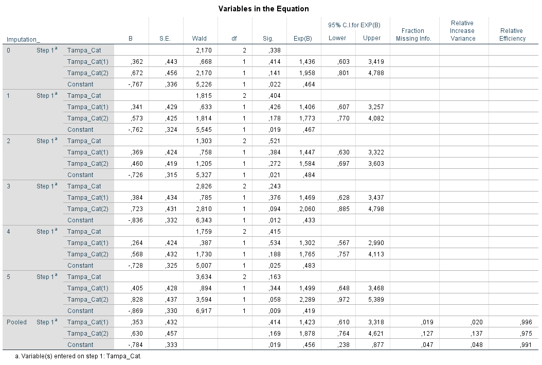
Figure 6.1: Logistic Regresion with an independent categorical variable.
There are several procedures to derive a pooled p-value for categorical variables, the pooled sampling variance or D1 method, the multiple parameter Wald test or D2 method, and the Meng and Rubin pooling procedure (Van Buuren (2018); Enders (2010); Eekhout, Wiel, and Heymans (2017); Meng and Rubin (1992); Mistler (2013); Marshall et al. (2009)). A more simple procedures to derive a pooled p-value for the overall Wald test is just taking the median of the p-values from the overall Wald test of all imputed data sets, this rule is called the Median P Rule (MPR) (Eekhout, Wiel, and Heymans (2017)). These methods can be performed in R.
6.2 Logistic regression with a categorical variable in R
Pooling of categorical variables can be done by using the psfmi package. The package contains a function called psfmi_lr for pooling of logistic regression models and psfmi_coxr, to pool right censored Cox regression models. Install the package and run the following code to pool the logistic regression model with as independent variable the categorical Tampa scale variable and as outcome the Radiation variable. To derive the pooled p-value for the overall Wald test, the D1 method is used. Other settings that can be used for method=, are “D2” for the D2 pooling method, “D3” for the Meng and Rubin method and “MPR” for the Median P Rule.
library(haven)
library(psfmi)
data <- read_sav(file="Backpain 150 Missing_Tampa_Cat Imp.sav")

pool_lr <- psfmi_lr(data=data, nimp=5, impvar="Imputation_", Outcome="Radiation",
  cat.predictors=c("Tampa_Cat"), method="D1")
pool_lr$RR_model
## $`Step 1 - no variables removed -`
## term estimate std.error statistic df p.value
## 1 (Intercept) -0.7843203 0.3329907 -2.3553819 129.04450 0.02001084
## 2 factor(Tampa_Cat)2 0.3526233 0.4319316 0.8163869 140.38462 0.41566202
## 3 factor(Tampa_Cat)3 0.6304326 0.4573147 1.3785532 87.29648 0.17155514
## OR lower.EXP upper.EXP
## 1 0.4564298 0.2361830 0.8820627
## 2 1.4227951 0.6057377 3.3419517
## 3 1.8784230 0.7569287 4.6615660Pooling a multivariable regression model that contains a mix of continuous, dichotomous and categorical variables can easily be performed with the psfmi_lr function. With the next code example, pooling is done in 10 multiple imputed datasets that are stored in the file lbpmilr (see ?lbpmilr for more information about the data set) . The relationship with the outcome variable “Chronic” is estimated, using a model with 2 dichotomous, 4 continuous and 2 categorical variables. The method to obtain a pooled p-value for the categorical variables is the D3 or Meng and Rubin method, indicated by method="D3". To obtain a pooled p-value for continuous and dichotomous variables Rubin’s Rules are used.
library(psfmi)

pool_lr <- psfmi_lr(data=lbpmilr, nimp=10, impvar="Impnr", Outcome="Chronic",
  predictors=c("Gender", "Smoking", "Function", "JobControl", "JobDemands",
  "SocialSupport"), cat.predictors = c("Carrying", "Satisfaction"),
  method="D3")
pool_lr$RR_model
## $`Step 1 - no variables removed -`
## term estimate std.error statistic df
## 1 (Intercept) -2.298884156 2.70946463 -0.84846435 131.80215
## 2 Gender -0.287716530 0.45800040 -0.62820147 138.79112
## 3 Smoking -0.024470165 0.37611364 -0.06506056 141.52168
## 4 Function -0.081066575 0.05051515 -1.60479742 123.41654
## 5 JobControl 0.002706353 0.02145167 0.12616047 119.96270
## 6 JobDemands 0.017142705 0.04116611 0.41642764 124.59855
## 7 SocialSupport 0.068131905 0.06095760 1.11769335 139.47522
## 8 factor(Carrying)2 1.372404083 0.53685785 2.55636402 109.96849
## 9 factor(Carrying)3 2.225494978 0.56415125 3.94485517 135.14483
## 10 factor(Satisfaction)2 -0.535017938 0.48487281 -1.10341914 100.59601
## 11 factor(Satisfaction)3 -1.048782938 0.60133404 -1.74409374 97.98729
## p.value OR lower.EXP upper.EXP
## 1 0.3977177144 0.1003708 0.0004719925 21.344180
## 2 0.5309043257 0.7499742 0.3032260550 1.854924
## 3 0.9482175928 0.9758268 0.4639412567 2.052497
## 4 0.1110943286 0.9221323 0.8343895859 1.019102
## 5 0.8998160992 1.0027100 0.9610137113 1.046215
## 6 0.6778135681 1.0172905 0.9376929799 1.103645
## 7 0.2656195026 1.0705065 0.9489601251 1.207621
## 8 0.0119415357 3.9448230 1.3613467275 11.431054
## 9 0.0001277054 9.2580642 3.0337158431 28.253059
## 10 0.2724777817 0.5856588 0.2238180139 1.532478
## 11 0.0842786793 0.3503639 0.1062338262 1.155516pool_lr$multiparm## $`Step 1 - no variables removed -`
## p-values D3 F-statistic
## Gender 0.5395154947 0.376623728
## Smoking 0.9578727441 0.002790571
## Function 0.0994785556 2.720351227
## JobControl 0.8893112153 0.019392026
## JobDemands 0.6749011364 0.176089120
## SocialSupport 0.2584423067 1.277387008
## factor(Carrying) 0.0002628256 8.320616618
## factor(Satisfaction) 0.2034079261 1.596048233In the table that is the pooled p-values can be found for all variables, including the categorical variables that are pooled by the Meng and Rubin or D3 method.
6.3 Cox Regression with a categorical variable in R
With the function psfmi_coxrit is also available to obtain overall pooled p-values for categorical variables in Cox regression models. All pooling methods can be applied, except for the Meng and Rubin procedure. The Meng and Rubin procedure is not recommended to use for Cox regression models (Marshall et al. (2009)).
To pool a Cox regression model with a mix of continuous and dichotomous variables and 1 categorical variable over 10 imputed datasets (see ?psfmi::lbpmicox for more information on the dataset) use the following code:
library(psfmi)

pool_coxr <- psfmi_coxr(data=lbpmicox, nimp=10, impvar="Impnr", time="Time", status="Status",
  predictors=c("Duration", "Radiation", "Onset", "Function", "Age",
  "Previous", "Tampascale", "JobControl", "JobDemand", "Social"),
  cat.predictors=c("Expect_cat"), method="D1")
pool_coxr$RR_model
## $`Step 1 - no variables removed -`
## term estimate std.error statistic df p.value
## 1 Duration -0.007783573 0.003994353 -1.9486444 178.4911 0.052905679
## 2 Radiation -0.074780449 0.153355337 -0.4876286 178.9568 0.626409768
## 3 Onset -0.093662790 0.175923953 -0.5324050 178.9837 0.595105843
## 4 Function 0.043898605 0.016858458 2.6039514 177.8688 0.009994408
## 5 Age -0.008894365 0.007706700 -1.1541081 178.4243 0.249999346
## 6 Previous -0.099450041 0.199199462 -0.4992485 178.2878 0.618219792
## 7 Tampascale -0.023507309 0.013833192 -1.6993409 167.8956 0.091106980
## 8 JobControl -0.008335826 0.008327722 -1.0009731 178.8756 0.318191958
## 9 JobDemand -0.021797568 0.015502737 -1.4060465 178.7206 0.161446545
## 10 Social -0.051460196 0.024886468 -2.0677983 178.7147 0.040099732
## 11 factor(Expect_cat)2 0.243470041 0.230764671 1.0550577 178.5326 0.292824622
## 12 factor(Expect_cat)3 0.227934593 0.200197639 1.1385479 178.8455 0.256414596
## HR lower.EXP upper.EXP
## 1 0.9922466 0.9844563 1.0000987
## 2 0.9279472 0.6856432 1.2558806
## 3 0.9105898 0.6435119 1.2885134
## 4 1.0448764 1.0106870 1.0802224
## 5 0.9911451 0.9761858 1.0063336
## 6 0.9053352 0.6110710 1.3413037
## 7 0.9767668 0.9504529 1.0038093
## 8 0.9916988 0.9755352 1.0081303
## 9 0.9784383 0.9489591 1.0088332
## 10 0.9498415 0.9043224 0.9976517
## 11 1.2756681 0.8090397 2.0114329
## 12 1.2560032 0.8460991 1.8644908pool_coxr$multiparm## $`Step 1 - no variables removed -`
## p-values D1 F-statistic
## Duration 0.05133866 3.7972150
## Radiation 0.62581293 0.2377817
## Onset 0.59444553 0.2834551
## Function 0.00921711 6.7805627
## Age 0.24845677 1.3319656
## Previous 0.61760484 0.2492491
## Tampascale 0.08939452 2.8877596
## JobControl 0.31683987 1.0019472
## JobDemand 0.15971062 1.9769667
## Social 0.03865924 4.2757898
## factor(Expect_cat) 0.48303066 0.7276753The pooled p-values according to method “D1” are shown in the last table.For more information about pooling possibilities of logistic and Cox regression models with the psfmi package see ?psfmi::psfmi_lr or ?psfmi::psfmi_coxr.
6.4 Variable selection
Prediction models are frequently developed by using selection procedures in logistic and Cox regression models. As a selection procedure, backward selection is generally recommended (Moons et al. (2015)). Variable selection in multiple imputed data sets may be challenging. When you apply variable selection in each imputed data set, different variables may be selected between imputed data sets. The question is than what is the best procedure to merge these different selected models into one final model. Wood (Wood, White, and Royston (2008)) showed that the best choice to select variables from multiply imputed data sets is to start your selection procedure from the pooled model. It is possible to do this in SPSS when the model includes continuous and dichotomous variables. This is however not possible in SPSS when the model contains categorical variables. Because categorical variables are estimated and selected by using an overall Wald Chi-square value and as we have seen in the previous paragraphs that that is not possible in SPSS. This is possible with the psfmi package, where you can choose between backward or forward selection.
6.4.1 Variable Selection with Logistic Regression models in R
Variable selection can be applied by using different methods to obtain pooled p-values and to select on basis of these pooled p-values. These methods were introduced in paragraph 6.1 and 6.2 and are called the “D1”, “D2”, “D3” (Meng and Rubin) and “MPR” (Median P Rule). Variable selection from the multivariable model that was pooled in paragraph 6.2 can be done by using the following settings in the psfmi function, method is “D1”, a p-value of 0.05 as selection criterion and direction=“BW” for backward selection.
library(psfmi)

pool_lr <- psfmi_lr(data=lbpmilr, nimp=10, impvar="Impnr", Outcome="Chronic",
  predictors=c("Gender", "Smoking", "Function", "JobControl", "JobDemands",
  "SocialSupport"), cat.predictors = c("Carrying", "Satisfaction"),
  p.crit = 0.05, method="D1", direction="BW")
## Removed at Step 1 is - Smoking## Removed at Step 2 is - JobControl## Removed at Step 3 is - JobDemands## Removed at Step 4 is - Gender## Removed at Step 5 is - SocialSupport## Removed at Step 6 is - factor(Satisfaction)## Removed at Step 7 is - Function##
## Selection correctly terminated,
## No more variables removed from the modelpool_lr$RR_model## $`Step 1 - removal - Smoking`
## term estimate std.error statistic df
## 1 (Intercept) -2.298884156 2.70946463 -0.84846435 131.80215
## 2 Gender -0.287716530 0.45800040 -0.62820147 138.79112
## 3 Smoking -0.024470165 0.37611364 -0.06506056 141.52168
## 4 Function -0.081066575 0.05051515 -1.60479742 123.41654
## 5 JobControl 0.002706353 0.02145167 0.12616047 119.96270
## 6 JobDemands 0.017142705 0.04116611 0.41642764 124.59855
## 7 SocialSupport 0.068131905 0.06095760 1.11769335 139.47522
## 8 factor(Carrying)2 1.372404083 0.53685785 2.55636402 109.96849
## 9 factor(Carrying)3 2.225494978 0.56415125 3.94485517 135.14483
## 10 factor(Satisfaction)2 -0.535017938 0.48487281 -1.10341914 100.59601
## 11 factor(Satisfaction)3 -1.048782938 0.60133404 -1.74409374 97.98729
## p.value OR lower.EXP upper.EXP
## 1 0.3977177144 0.1003708 0.0004719925 21.344180
## 2 0.5309043257 0.7499742 0.3032260550 1.854924
## 3 0.9482175928 0.9758268 0.4639412567 2.052497
## 4 0.1110943286 0.9221323 0.8343895859 1.019102
## 5 0.8998160992 1.0027100 0.9610137113 1.046215
## 6 0.6778135681 1.0172905 0.9376929799 1.103645
## 7 0.2656195026 1.0705065 0.9489601251 1.207621
## 8 0.0119415357 3.9448230 1.3613467275 11.431054
## 9 0.0001277054 9.2580642 3.0337158431 28.253059
## 10 0.2724777817 0.5856588 0.2238180139 1.532478
## 11 0.0842786793 0.3503639 0.1062338262 1.155516
##
## $`Step 2 - removal - JobControl`
## term estimate std.error statistic df
## 1 (Intercept) -2.305291511 2.70502030 -0.8522271 132.7674
## 2 Gender -0.289071210 0.45750446 -0.6318435 139.7058
## 3 Function -0.081272411 0.05045719 -1.6107202 123.8316
## 4 JobControl 0.002692794 0.02143825 0.1256069 120.6760
## 5 JobDemands 0.017116963 0.04115819 0.4158823 125.4520
## 6 SocialSupport 0.068160926 0.06094494 1.1184017 140.4387
## 7 factor(Carrying)2 1.366848152 0.53193989 2.5695538 110.2454
## 8 factor(Carrying)3 2.221969432 0.56285759 3.9476583 136.1990
## 9 factor(Satisfaction)2 -0.531622312 0.48184969 -1.1032949 102.7084
## 10 factor(Satisfaction)3 -1.042673978 0.59418183 -1.7548062 100.6774
## p.value OR lower.EXP upper.EXP
## 1 0.3956227615 0.09972972 0.0004732897 21.014652
## 2 0.5285217348 0.74895887 0.3031284264 1.850501
## 3 0.1097868616 0.92194251 0.8343163285 1.018772
## 4 0.9002520845 1.00269642 0.9610286713 1.046171
## 5 0.6782067036 1.01726430 0.9376886234 1.103593
## 6 0.2653048850 1.07053757 0.9490182791 1.207617
## 7 0.0115181418 3.92296659 1.3671034621 11.257134
## 8 0.0001259448 9.22548194 3.0310191915 28.079505
## 9 0.2724774479 0.58765084 0.2259842957 1.528131
## 10 0.0823346846 0.35251081 0.1084553533 1.145761
##
## $`Step 3 - removal - JobDemands`
## term estimate std.error statistic df p.value
## 1 (Intercept) -2.10777898 2.23946055 -0.9411994 127.2701 0.3483857231
## 2 Gender -0.30388145 0.44724067 -0.6794584 136.6301 0.4979969233
## 3 Function -0.07997909 0.04960562 -1.6122990 121.6983 0.1094872554
## 4 JobDemands 0.01687441 0.04116528 0.4099186 124.2023 0.6825718579
## 5 SocialSupport 0.06664849 0.05977564 1.1149774 140.9667 0.2667573500
## 6 factor(Carrying)2 1.36281048 0.53184025 2.5624433 110.3218 0.0117418616
## 7 factor(Carrying)3 2.22055062 0.56233236 3.9488224 136.6557 0.0001252143
## 8 factor(Satisfaction)2 -0.52782215 0.48058337 -1.0982947 103.4591 0.2746252649
## 9 factor(Satisfaction)3 -1.04815781 0.59363812 -1.7656511 100.3204 0.0804968712
## OR lower.EXP upper.EXP
## 1 0.1215075 0.001445678 10.212565
## 2 0.7379483 0.304741791 1.786981
## 3 0.9231356 0.836791106 1.018390
## 4 1.0170176 0.937440584 1.103350
## 5 1.0689197 0.949780762 1.203003
## 6 3.9071589 1.361874602 11.209469
## 7 9.2124020 3.029968117 28.009652
## 8 0.5898883 0.227433895 1.529975
## 9 0.3505830 0.107973132 1.138324
##
## $`Step 4 - removal - Gender`
## term estimate std.error statistic df
## 1 (Intercept) -1.49026863 1.62421415 -0.9175321 143.10301
## 2 Gender -0.33380360 0.43803902 -0.7620408 140.12403
## 3 Function -0.08145016 0.04945028 -1.6471123 121.73159
## 4 SocialSupport 0.06652752 0.05975615 1.1133167 142.13039
## 5 factor(Carrying)2 1.34476016 0.52615210 2.5558392 114.70848
## 6 factor(Carrying)3 2.19935239 0.55690548 3.9492382 139.54866
## 7 factor(Satisfaction)2 -0.51163883 0.47725869 -1.0720367 105.16687
## 8 factor(Satisfaction)3 -1.03097451 0.59335708 -1.7375280 98.73457
## p.value OR lower.EXP upper.EXP
## 1 0.3604076635 0.2253121 0.009087819 5.586110
## 2 0.4473164214 0.7161944 0.301247347 1.702702
## 3 0.1021140654 0.9217786 0.835818255 1.016580
## 4 0.2674517413 1.0687904 0.949710424 1.202801
## 5 0.0119008226 3.8372661 1.353272806 10.880741
## 6 0.0001238953 9.0191707 2.999031197 27.123906
## 7 0.2861574758 0.5995123 0.232715839 1.544437
## 8 0.0854121555 0.3566592 0.109880393 1.157675
##
## $`Step 5 - removal - SocialSupport`
## term estimate std.error statistic df p.value
## 1 (Intercept) -1.83426824 1.55119482 -1.182487 145.7793 0.2389374534
## 2 Function -0.08461791 0.04915512 -1.721446 123.9954 0.0876637699
## 3 SocialSupport 0.06943358 0.05904870 1.175870 144.0310 0.2415868450
## 4 factor(Carrying)2 1.41737344 0.51529645 2.750598 117.0798 0.0068942977
## 5 factor(Carrying)3 2.21168140 0.55667467 3.973023 139.3247 0.0001133678
## 6 factor(Satisfaction)2 -0.48309188 0.47389039 -1.019417 107.0790 0.3103028134
## 7 factor(Satisfaction)3 -0.98823853 0.58774671 -1.681402 100.1208 0.0958017791
## OR lower.EXP upper.EXP
## 1 0.1597303 0.007446552 3.426255
## 2 0.9188633 0.833676611 1.012755
## 3 1.0719009 0.953819923 1.204600
## 4 4.1262683 1.487152303 11.448787
## 5 9.1310564 3.037573950 27.448284
## 6 0.6168731 0.241106537 1.578275
## 7 0.3722318 0.115985043 1.194607
##
## $`Step 6 - removal - factor(Satisfaction)`
## term estimate std.error statistic df p.value
## 1 (Intercept) -0.2562418 0.80887524 -0.3167878 129.2721 0.7519156211
## 2 Function -0.0800438 0.04892178 -1.6361587 123.5788 0.1043507473
## 3 factor(Carrying)2 1.3950528 0.51127910 2.7285544 120.4119 0.0073142359
## 4 factor(Carrying)3 2.1630529 0.55215055 3.9175056 142.2884 0.0001384142
## 5 factor(Satisfaction)2 -0.4668701 0.46837359 -0.9967901 111.6805 0.3210212648
## 6 factor(Satisfaction)3 -0.9566312 0.58102627 -1.6464508 104.6421 0.1026711663
## OR lower.EXP upper.EXP
## 1 0.7739548 0.1562045 3.834756
## 2 0.9230759 0.8378829 1.016931
## 3 4.0351878 1.4663716 11.104102
## 4 8.6976501 2.9199737 25.907465
## 5 0.6269615 0.2478525 1.585946
## 6 0.3841850 0.1213902 1.215898
##
## $`Step 7 - removal - Function`
## term estimate std.error statistic df p.value
## 1 (Intercept) -0.75217049 0.72090546 -1.043369 133.0852 0.2986689258
## 2 Function -0.06808302 0.04716385 -1.443542 133.8147 0.1512047478
## 3 factor(Carrying)2 1.35182349 0.50310305 2.686971 123.4131 0.0082044805
## 4 factor(Carrying)3 1.96318987 0.53229181 3.688184 140.7366 0.0003217835
## OR lower.EXP upper.EXP
## 1 0.4713424 0.1132582 1.961568
## 2 0.9341829 0.8509805 1.025520
## 3 3.8644659 1.4276004 10.460979
## 4 7.1220091 2.4864808 20.399519
##
## $`Step 8 - removal - ended`
## term estimate std.error statistic df p.value
## 1 (Intercept) -1.635860 0.3984964 -4.105081 136.2077 6.928373e-05
## 2 factor(Carrying)2 1.476823 0.4956309 2.979683 121.6077 3.484942e-03
## 3 factor(Carrying)3 2.275099 0.4885529 4.656812 146.4497 7.141622e-06
## OR lower.EXP upper.EXP
## 1 0.1947848 0.08857552 0.4283478
## 2 4.3790126 1.64154952 11.6814945
## 3 9.7288803 3.70459592 25.5496455pool_lr$multiparm## $`Step 1 - removal - Smoking`
## p-values D1 F-statistic
## Gender 0.5299231920 0.394637093
## Smoking 0.9481280019 0.004232877
## Function 0.1091413298 2.575374761
## JobControl 0.8996644949 0.015916465
## JobDemands 0.6772549331 0.173411982
## SocialSupport 0.2637803526 1.249238433
## factor(Carrying) 0.0005542759 7.527987156
## factor(Satisfaction) 0.2067375869 1.579009536
##
## $`Step 2 - removal - JobControl`
## p-values D1 F-statistic
## Gender 0.5275409424 0.3992262
## Function 0.1078571780 2.5944195
## JobControl 0.9001024794 0.0157771
## JobDemands 0.6776530407 0.1729581
## SocialSupport 0.2634774617 1.2508223
## factor(Carrying) 0.0005565268 7.5250676
## factor(Satisfaction) 0.2037151384 1.5936489
##
## $`Step 3 - removal - JobDemands`
## p-values D1 F-statistic
## Gender 0.4969551605 0.4616638
## Function 0.1076277995 2.5995080
## JobDemands 0.6820414543 0.1680332
## SocialSupport 0.2649497612 1.2431746
## factor(Carrying) 0.0005640488 7.5138290
## factor(Satisfaction) 0.1992050886 1.6160862
##
## $`Step 4 - removal - Gender`
## p-values D1 F-statistic
## Gender 0.4461198510 0.5807062
## Function 0.1002912385 2.7129788
## SocialSupport 0.2656576474 1.2394741
## factor(Carrying) 0.0005646679 7.5087416
## factor(Satisfaction) 0.2089058935 1.5685193
##
## $`Step 5 - removal - SocialSupport`
## p-values D1 F-statistic
## Function 0.0858545802 2.963378
## SocialSupport 0.2397178007 1.382670
## factor(Carrying) 0.0004580153 7.715752
## factor(Satisfaction) 0.2316077904 1.465004
##
## $`Step 6 - removal - factor(Satisfaction)`
## p-values D1 F-statistic
## Function 0.1025484398 2.677015
## factor(Carrying) 0.0005943588 7.453469
## factor(Satisfaction) 0.2472398361 1.399255
##
## $`Step 7 - removal - Function`
## p-values D1 F-statistic
## Function 0.149295714 2.083815
## factor(Carrying) 0.001286134 6.679181
##
## $`Step 8 - removal - ended`
## p-values D1 F-statistic
## factor(Carrying) 3.177679e-05 10.40568See ?psfmi::psfmi_lr for other possibilities during variable selection with the psfmi_lrfunction like forcing variables in the model during variable selection or variable selection with interaction terms.
6.4.2 Variable Selection with Cox Regression models in R
We can apply backward variable selection for a Cox regression model using the “D1” method, a p-value of 0.05 as selection criterium and direction = “BW” for backward selection.
library(psfmi)

pool_coxr <- psfmi_coxr(data=lbpmicox, nimp=10, impvar="Impnr", time="Time", status="Status",
  predictors=c("Duration", "Radiation", "Onset", "Function", "Age",
  "Previous", "Tampascale", "JobControl", "JobDemand", "Social"),
  cat.predictors=c("Expect_cat"), p.crit = 0.05, method="D1", direction = "BW")
## Removed at Step 1 is - Radiation## Removed at Step 2 is - Previous## Removed at Step 3 is - Onset## Removed at Step 4 is - factor(Expect_cat)## Removed at Step 5 is - JobControl## Removed at Step 6 is - Age## Removed at Step 7 is - JobDemand## Removed at Step 8 is - Tampascale##
## Selection correctly terminated,
## No more variables removed from the modelpool_coxr$RR_model## $`Step 1 - removal - Radiation`
## term estimate std.error statistic df p.value
## 1 Duration -0.007783573 0.003994353 -1.9486444 178.4911 0.052905679
## 2 Radiation -0.074780449 0.153355337 -0.4876286 178.9568 0.626409768
## 3 Onset -0.093662790 0.175923953 -0.5324050 178.9837 0.595105843
## 4 Function 0.043898605 0.016858458 2.6039514 177.8688 0.009994408
## 5 Age -0.008894365 0.007706700 -1.1541081 178.4243 0.249999346
## 6 Previous -0.099450041 0.199199462 -0.4992485 178.2878 0.618219792
## 7 Tampascale -0.023507309 0.013833192 -1.6993409 167.8956 0.091106980
## 8 JobControl -0.008335826 0.008327722 -1.0009731 178.8756 0.318191958
## 9 JobDemand -0.021797568 0.015502737 -1.4060465 178.7206 0.161446545
## 10 Social -0.051460196 0.024886468 -2.0677983 178.7147 0.040099732
## 11 factor(Expect_cat)2 0.243470041 0.230764671 1.0550577 178.5326 0.292824622
## 12 factor(Expect_cat)3 0.227934593 0.200197639 1.1385479 178.8455 0.256414596
## HR lower.EXP upper.EXP
## 1 0.9922466 0.9844563 1.0000987
## 2 0.9279472 0.6856432 1.2558806
## 3 0.9105898 0.6435119 1.2885134
## 4 1.0448764 1.0106870 1.0802224
## 5 0.9911451 0.9761858 1.0063336
## 6 0.9053352 0.6110710 1.3413037
## 7 0.9767668 0.9504529 1.0038093
## 8 0.9916988 0.9755352 1.0081303
## 9 0.9784383 0.9489591 1.0088332
## 10 0.9498415 0.9043224 0.9976517
## 11 1.2756681 0.8090397 2.0114329
## 12 1.2560032 0.8460991 1.8644908
##
## $`Step 2 - removal - Previous`
## term estimate std.error statistic df p.value
## 1 Duration -0.007911303 0.003990849 -1.9823609 179.4621 0.048965042
## 2 Onset -0.090681699 0.175646663 -0.5162734 179.9838 0.606297177
## 3 Function 0.045581711 0.016456535 2.7698244 178.8970 0.006200509
## 4 Age -0.008886199 0.007716358 -1.1516053 179.3925 0.251015778
## 5 Previous -0.089344066 0.198134429 -0.4509265 179.2517 0.652587517
## 6 Tampascale -0.023515751 0.013796782 -1.7044374 169.0769 0.090136296
## 7 JobControl -0.008656570 0.008261454 -1.0478264 179.8551 0.296124640
## 8 JobDemand -0.021603021 0.015474101 -1.3960760 179.7177 0.164413739
## 9 Social -0.050888762 0.024839258 -2.0487231 179.6993 0.041943257
## 10 factor(Expect_cat)2 0.266587552 0.226163448 1.1787385 179.4493 0.240062927
## 11 factor(Expect_cat)3 0.244048620 0.197600903 1.2350582 179.8196 0.218420136
## HR lower.EXP upper.EXP
## 1 0.9921199 0.9843376 0.9999637
## 2 0.9133084 0.6457949 1.2916364
## 3 1.0466365 1.0131941 1.0811828
## 4 0.9911532 0.9761757 1.0063604
## 5 0.9145309 0.6185854 1.3520635
## 6 0.9767586 0.9505145 1.0037273
## 7 0.9913808 0.9753505 1.0076746
## 8 0.9786287 0.9491985 1.0089713
## 9 0.9503844 0.9049253 0.9981271
## 10 1.3055019 0.8355255 2.0398362
## 11 1.2764064 0.8642733 1.8850672
##
## $`Step 3 - removal - Onset`
## term estimate std.error statistic df p.value
## 1 Duration -0.007670615 0.003954661 -1.9396391 180.4776 0.053982519
## 2 Onset -0.085934310 0.175259961 -0.4903248 180.9868 0.624497956
## 3 Function 0.045425448 0.016419427 2.7665672 180.0073 0.006256421
## 4 Age -0.009251228 0.007668918 -1.2063278 180.3254 0.229271416
## 5 Tampascale -0.023083288 0.013751202 -1.6786379 171.5059 0.095043723
## 6 JobControl -0.009078357 0.008203584 -1.1066330 180.8938 0.269922092
## 7 JobDemand -0.022054011 0.015433231 -1.4289951 180.7873 0.154731207
## 8 Social -0.051613208 0.024787910 -2.0821928 180.6802 0.038733647
## 9 factor(Expect_cat)2 0.263984652 0.225835616 1.1689239 180.5173 0.243975561
## 10 factor(Expect_cat)3 0.252951520 0.196441942 1.2876655 180.7735 0.199508426
## HR lower.EXP upper.EXP
## 1 0.9923587 0.9846452 1.0001327
## 2 0.9176545 0.6493718 1.2967761
## 3 1.0464730 1.0131113 1.0809332
## 4 0.9907914 0.9759113 1.0058985
## 5 0.9771811 0.9510138 1.0040684
## 6 0.9909627 0.9750511 1.0071340
## 7 0.9781874 0.9488482 1.0084338
## 8 0.9496961 0.9043632 0.9973015
## 9 1.3021082 0.8339077 2.0331815
## 10 1.2878208 0.8740108 1.8975538
##
## $`Step 4 - removal - factor(Expect_cat)`
## term estimate std.error statistic df p.value
## 1 Duration -0.007780265 0.003947974 -1.970698 181.4407 0.050279458
## 2 Function 0.045346889 0.016439010 2.758493 180.9830 0.006403233
## 3 Age -0.009010544 0.007677657 -1.173606 181.3178 0.242092185
## 4 Tampascale -0.023328570 0.013725411 -1.699663 172.5549 0.090996269
## 5 JobControl -0.008772204 0.008162829 -1.074652 181.8930 0.283953857
## 6 JobDemand -0.021960209 0.015421007 -1.424045 181.7750 0.156147775
## 7 Social -0.052455019 0.024656573 -2.127425 181.6638 0.034733741
## 8 factor(Expect_cat)2 0.265521832 0.225807983 1.175874 181.5127 0.241185025
## 9 factor(Expect_cat)3 0.252304256 0.196302201 1.285285 181.7729 0.200327923
## HR lower.EXP upper.EXP
## 1 0.9922499 0.9845505 1.0000096
## 2 1.0463908 1.0129938 1.0808888
## 3 0.9910299 0.9761299 1.0061574
## 4 0.9769414 0.9508301 1.0037698
## 5 0.9912662 0.9754287 1.0073608
## 6 0.9782792 0.9489612 1.0085029
## 7 0.9488970 0.9038380 0.9962023
## 8 1.3041113 0.8352499 2.0361647
## 9 1.2869876 0.8736987 1.8957760
##
## $`Step 5 - removal - JobControl`
## term estimate std.error statistic df p.value HR
## 1 Duration -0.007482473 0.003904692 -1.916277 183.5758 0.056883350 0.9925455
## 2 Function 0.047555491 0.016491699 2.883602 183.3303 0.004402089 1.0487044
## 3 Age -0.008142310 0.007553982 -1.077883 183.4896 0.282500924 0.9918907
## 4 Tampascale -0.021077061 0.013554581 -1.554977 177.0415 0.121737375 0.9791435
## 5 JobControl -0.008336947 0.008167415 -1.020757 183.9129 0.308710372 0.9916977
## 6 JobDemand -0.020908601 0.015394478 -1.358188 183.8088 0.176068636 0.9793085
## 7 Social -0.052535961 0.024367155 -2.156015 183.7044 0.032382844 0.9488202
## lower.EXP upper.EXP
## 1 0.9849284 1.0002214
## 2 1.0151309 1.0833883
## 3 0.9772174 1.0067844
## 4 0.9532993 1.0056884
## 5 0.9758457 1.0078072
## 6 0.9500115 1.0095089
## 7 0.9042843 0.9955494
##
## $`Step 6 - removal - Age`
## term estimate std.error statistic df p.value HR
## 1 Duration -0.007053937 0.003875984 -1.819909 184.5632 0.070393010 0.9929709
## 2 Function 0.047528931 0.016535905 2.874287 184.2430 0.004525734 1.0486765
## 3 Age -0.007973471 0.007584308 -1.051312 184.4663 0.294490761 0.9920582
## 4 Tampascale -0.021050280 0.013619183 -1.545635 177.2980 0.123975890 0.9791697
## 5 JobDemand -0.019220676 0.015372253 -1.250349 184.7943 0.212753181 0.9809629
## 6 Social -0.060880870 0.022865188 -2.662601 184.6947 0.008438263 0.9409353
## lower.EXP upper.EXP
## 1 0.9854067 1.0005932
## 2 1.0150165 1.0834528
## 3 0.9773244 1.0070142
## 4 0.9532035 1.0058433
## 5 0.9516591 1.0111689
## 6 0.8994324 0.9843534
##
## $`Step 7 - removal - JobDemand`
## term estimate std.error statistic df p.value HR
## 1 Duration -0.007865649 0.003799883 -2.069971 185.6839 0.039839147 0.9921652
## 2 Function 0.048080451 0.016611851 2.894346 185.4604 0.004255196 1.0492551
## 3 Tampascale -0.018502738 0.013317643 -1.389340 180.2673 0.166443021 0.9816674
## 4 JobDemand -0.017743416 0.015260646 -1.162691 185.8081 0.246445996 0.9824131
## 5 Social -0.060274490 0.022898863 -2.632205 185.8169 0.009196667 0.9415061
## lower.EXP upper.EXP
## 1 0.9847553 0.9996309
## 2 1.0154257 1.0842114
## 3 0.9562066 1.0078061
## 4 0.9532769 1.0124397
## 5 0.8999198 0.9850141
##
## $`Step 8 - removal - Tampascale`
## term estimate std.error statistic df p.value HR
## 1 Duration -0.008092142 0.003783744 -2.138660 186.5610 0.033763716 0.9919405
## 2 Function 0.048380567 0.016396389 2.950684 186.3046 0.003577911 1.0495700
## 3 Tampascale -0.021112332 0.013189846 -1.600650 180.8169 0.111200083 0.9791090
## 4 Social -0.056501637 0.022696621 -2.489429 186.6223 0.013669630 0.9450649
## lower.EXP upper.EXP
## 1 0.9845638 0.9993725
## 2 1.0161634 1.0840749
## 3 0.9539556 1.0049256
## 4 0.9036831 0.9883418
##
## $`Step 9 - removal - ended`
## term estimate std.error statistic df p.value HR
## 1 Duration -0.007605055 0.003742491 -2.032084 188.0122 0.0435521395 0.9924238
## 2 Function 0.056490633 0.015414714 3.664722 188.0122 0.0003219893 1.0581167
## 3 Social -0.051992380 0.022611457 -2.299382 188.0122 0.0225821313 0.9493361
## lower.EXP upper.EXP
## 1 0.9851240 0.9997776
## 2 1.0264257 1.0907861
## 3 0.9079217 0.9926396pool_coxr$multiparm## $`Step 1 - removal - Radiation`
## p-values D1 F-statistic
## Duration 0.05133866 3.7972150
## Radiation 0.62581293 0.2377817
## Onset 0.59444553 0.2834551
## Function 0.00921711 6.7805627
## Age 0.24845677 1.3319656
## Previous 0.61760484 0.2492491
## Tampascale 0.08939452 2.8877596
## JobControl 0.31683987 1.0019472
## JobDemand 0.15971062 1.9769667
## Social 0.03865924 4.2757898
## factor(Expect_cat) 0.48303066 0.7276753
##
## $`Step 2 - removal - Previous`
## p-values D1 F-statistic
## Duration 0.047439666 3.9297548
## Onset 0.605663477 0.2665382
## Function 0.005609748 7.6719271
## Age 0.249484299 1.3261948
## Previous 0.652043040 0.2033347
## Tampascale 0.088433945 2.9051067
## JobControl 0.294718661 1.0979402
## JobDemand 0.162691906 1.9490282
## Social 0.040489472 4.1972664
## factor(Expect_cat) 0.413557823 0.8829582
##
## $`Step 3 - removal - Onset`
## p-values D1 F-statistic
## Duration 0.052424344 3.7621998
## Onset 0.623904064 0.2404184
## Function 0.005665895 7.6538941
## Age 0.227692389 1.4552266
## Tampascale 0.093331539 2.8178252
## JobControl 0.268452683 1.2246366
## JobDemand 0.153005830 2.0420269
## Social 0.037325158 4.3355268
## factor(Expect_cat) 0.398682504 0.9195901
##
## $`Step 4 - removal - factor(Expect_cat)`
## p-values D1 F-statistic
## Duration 0.048759275 3.8836508
## Function 0.005807806 7.6092824
## Age 0.240554119 1.3773510
## Tampascale 0.089300761 2.8888534
## JobControl 0.282530421 1.1548778
## JobDemand 0.154433617 2.0279044
## Social 0.033385062 4.5259387
## factor(Expect_cat) 0.397814846 0.9217688
##
## $`Step 5 - removal - JobControl`
## p-values D1 F-statistic
## Duration 0.055330339 3.672119
## Function 0.003931908 8.315158
## Age 0.281086598 1.161832
## Tampascale 0.120018618 2.417953
## JobControl 0.307369556 1.041945
## JobDemand 0.174404049 1.844676
## Social 0.031082697 4.648402
##
## $`Step 6 - removal - Age`
## p-values D1 F-statistic
## Duration 0.068773491 3.312068
## Function 0.004049852 8.261523
## Age 0.293116188 1.105256
## Tampascale 0.122270111 2.388986
## JobDemand 0.211172366 1.563372
## Social 0.007754059 7.089443
##
## $`Step 7 - removal - JobDemand`
## p-values D1 F-statistic
## Duration 0.038455309 4.284781
## Function 0.003799714 8.377242
## Tampascale 0.164776983 1.930266
## JobDemand 0.244955007 1.351850
## Social 0.008483332 6.928501
##
## $`Step 8 - removal - Tampascale`
## p-values D1 F-statistic
## Duration 0.032463658 4.573867
## Function 0.003171026 8.706537
## Tampascale 0.109508478 2.562082
## Social 0.012795066 6.197259
##
## $`Step 9 - removal - ended`
## p-values D1 F-statistic
## Duration 0.0421452034 4.129363
## Function 0.0002476079 13.430184
## Social 0.0214832491 5.2871586.5 Interaction terms in model
When the analysis model contains an interaction term, and one of the variables that is part of the interaction term contains missing data, it is important that the imputation procedure takes into account that different effects exist with the outcome for different categories of the effect modifier that is part of the interaction term. Otherwise the imputation model may not be consistent with the analysis model and this results in incorrect imputed values and biased coefficients and standard error estimates (Bartlett et al. (2015)).
For example, we may be interested in the relationship between (body)weight and blood pressure, with gender as effect modifier. The main aim of this model is to study the relationship between (body)weight and blood pressure (SBP) and whether this relationship depends on gender, i.e. is stronger or less strong for males compared to females. The analysis model is:
\[SBP = β{_0} + β{_1} * BodyWeight + β{_2} * Gender + β{_3} * BodyWeight * Gender\]
Assume now that there is missing data in the bodyweight variable. As a result, there will also be missing data in the interaction term between bodyweight and Gender.
When the imputation model consists of the following formula:
\[BodyWeight{_{mis}} = β{_0} + β{_1} * SBP + β{_2} * Gender\] The imputation model is not consistent with the analysis model and would therefore not be able to generate valid imputations. We have to use an imputation procedure that takes into account that the relationship between Bodyweight and Blood pressure depends on Gender. A solution is to impute the relationship between blood pressure and bodyweight separately for males and females. That way, you account for the possibility that the relationship between bodyweight and blood pressure differs between males and females and the imputed values can then differ too.
Imputation of interaction terms in SPSS
To impute the missing data in the Bodyweight variable to examine the relationship between bodyweight and blood pressure, in a model including the interaction between bodyweight and gender are explained in the next steps.
Step 1 Split the dataset by Gender.
Data -> Split File -> Compare Groups
Move the Gender variable to the window: Group based on, then click OK.
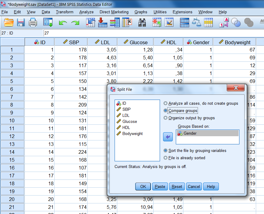
Figure 6.2: Bodyweight dataset with missing values in the Bodyweight variable.
Step 2 Perform Multiple Imputation. Use all variables in the imputation model, except the Gender variable. The Gender variable was used as a split variable and cannot be included in the imputation model. MI is now separately performed for Males and Females.
Step 3 Subsequently, turn on the split on the variable Imputation_ in the dataset with the imputed values. This will automatically turn off the split on Gender.
Step 4 Compute the Interaction term between Bodyweight and Gender via:
Transform -> Compute Variable
Step 5 Fit the regression model to Obtain Pooled results for the main analysis model.
For logistic or Cox regression models the same steps can be followed. For these models at step 4 it is not necessary to compute an interaction term. The inclusion of interaction terms in the model can be activated by first selecting 1 variable that is part of the interaction term, than pressing the Ctrl key and selecting the other variable at the same time. The >a*b> key will than be lighted and after you click on that button the interaction term is included in the model.
Imputation of interaction terms in R
The split file procedure that we used in SPSS in the previous paragraph to impute missing data and to take interaction terms into account can also be applied in R. First you have to split the data, impute the missing values, merge the data again and generate the interaction term in the dataset . Then results of the analysis model can be pooled. There is also another procedure in R that can be used. This procedure is called Substantive Model Compatible Fully Conditional Specification (SMC-FCS). This is a fairly complex procedure that can generate valid imputations by taking into account interaction terms. More about this procedure can be found in the technical paper of Bartlett et al.( 2015). To apply the procedure we need the smcfcs function which is available in the smcfs package (Bartlett, 2015). To get pooled analysis results we also have to install the mitoolspackage.
We are currently working on this Chapter.