4 Tidyverse 3: Review and practice
4.1 Presentation: Country Facts
First, we’ll look at the homework that you submitted. Teach me something about your country.
4.2 Review together: loading data, head(), tail()
This week is all about practice. I want to make sure you understand the basics before we start making charts, maps and websites.
Let’s clean some data together.
- Make a new file
- Save your file
- Load the Tidyverse
- … and let’s get started. Here’s a link to a data set:
https://opendata.swiss/de/dataset/lebendgeburten-nach-alter-der-mutter-geschlecht-des-kindes-und-kanton-1969-2023/resource/109ed5a9-9495-49be-ba7b-8e779aca5d3eYou can get the download link, usually, by finding the button, right clicking, and hitting “Copy link address”. This will be slightly different depending on your browser.
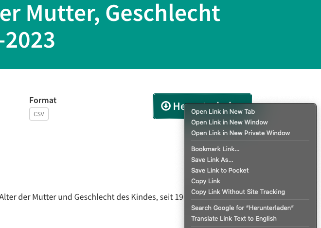
Figure 4.1: You need to make sure you have a link to the file you want.
- Download it into your project folder.
download.file("https://dam-api.bfs.admin.ch/hub/api/dam/assets/32007752/master", "input_data/births.csv")Note: On Windows, you need to make an adjustment. You need to add mode = "wb" to the download.file() function.
download.file("https://dam-api.bfs.admin.ch/hub/api/dam/assets/32007752/master", "input_data/births.csv", mode = "wb") - Load this data set into your R session
- Take a look at the first 20 rows of the data set. Can you figure out what each column is?
## # A tibble: 6 × 5
##    YEAR CANTON AGE_MOTHER SEX_CHILD OBS_VALUE
##   <dbl> <chr>  <chr>      <chr>         <dbl>
## 1  1969 CH     _T         T            102520
## 2  1969 CH     _T         F             49990
## 3  1969 CH     _T         M             52530
## 4  1969 CH     Y10T14     T                 6
## 5  1969 CH     Y10T14     F                 3
## 6 1969 CH Y10T14 M 3- Now look at the last 20 rows. What are some of the steps we’re going to have to take?
## # A tibble: 6 × 5
##    YEAR CANTON AGE_MOTHER SEX_CHILD OBS_VALUE
##   <dbl> <chr>  <chr>      <chr>         <dbl>
## 1  2023 26     Y60T64     T                 0
## 2  2023 26     Y60T64     F                 0
## 3  2023 26     Y60T64     M                 0
## 4  2023 26     Y65T69     T                 0
## 5  2023 26     Y65T69     F                 0
## 6  2023 26     Y65T69     M                 0
Can we guess what every column is?
4.3 Classwork: filter()
To review, the filter() function will sort out the data you want from the stuff you don’t. For example, if you only wanted a dataset for boys in Zürich in 1970, you could use the following code:
## # A tibble: 13 × 5
##     YEAR CANTON AGE_MOTHER SEX_CHILD OBS_VALUE
##    <dbl> <chr>  <chr>      <chr>         <dbl>
##  1  1970 1      _T         M              8330
##  2  1970 1      Y10T14     M                 0
##  3  1970 1      Y15T19     M               279
##  4  1970 1      Y20T24     M              2274
##  5  1970 1      Y25T29     M              3119
##  6  1970 1      Y30T34     M              1745
##  7  1970 1      Y35T39     M               768
##  8  1970 1      Y40T44     M               133
##  9  1970 1      Y45T49     M                12
## 10  1970 1      Y50T54     M                 0
## 11  1970 1      Y55T59     M                 0
## 12  1970 1      Y60T64     M                 0
## 13  1970 1      Y65T69     M                 0
Please answer the following questions: Your answer should be a code block that uses the filter() function to find the answer.
- How many babies were born in Vaud (Canton number 22) in 2020?
- How many girls were born in Zurich (Canton number 1) to mothers aged 30-34 in 2019?
- Between 2000 and 2020, How many years did Ticino (Canton number 21) have fewer than 1400 boys born?
- How many boys and girls were born in Switzerland in 2015?
4.4 Classwork: select(), rename(), mutate()
Let’s clean up the data set.
- TYPING IN ALL CAPS IS ANNOYING. Rename the columns to
year, canton, age_of_mother, sex_of_child, total_born. You can userename()orcolnames() <- c(). It should look like this:
## # A tibble: 10 × 5
##     year canton age_of_mother sex_of_child total_born
##    <dbl> <chr>  <chr>         <chr>             <dbl>
##  1  1969 CH     _T            T                102520
##  2  1969 CH     _T            F                 49990
##  3  1969 CH     _T            M                 52530
##  4  1969 CH     Y10T14        T                     6
##  5  1969 CH     Y10T14        F                     3
##  6  1969 CH     Y10T14        M                     3
##  7  1969 CH     Y15T19        T                  3648
##  8  1969 CH     Y15T19        F                  1780
##  9  1969 CH     Y15T19        M                  1868
## 10 1969 CH Y20T24 T 30230- Let’s say I don’t care about gender. I want to know the total number of children born in each Canton each year to mothers of different ages. Filter only the total number of children born, and discard the boy and girl counts. It should look like this:
## # A tibble: 10 × 5
##     year canton age_of_mother sex_of_child total_born
##    <dbl> <chr>  <chr>         <chr>             <dbl>
##  1  1969 CH     _T            T                102520
##  2  1969 CH     Y10T14        T                     6
##  3  1969 CH     Y15T19        T                  3648
##  4  1969 CH     Y20T24        T                 30230
##  5  1969 CH     Y25T29        T                 36206
##  6  1969 CH     Y30T34        T                 20479
##  7  1969 CH     Y35T39        T                  9077
##  8  1969 CH     Y40T44        T                  2633
##  9  1969 CH     Y45T49        T                   240
## 10 1969 CH Y50T54 T 1- Now that
sex_of_childcolumn is pretty useless, isn’t it? Let’s select() only the columns that we care about. It should look like this:
## # A tibble: 10 × 4
##     year canton age_of_mother total_born
##    <dbl> <chr>  <chr>              <dbl>
##  1  1969 CH     _T                102520
##  2  1969 CH     Y10T14                 6
##  3  1969 CH     Y15T19              3648
##  4  1969 CH     Y20T24             30230
##  5  1969 CH     Y25T29             36206
##  6  1969 CH     Y30T34             20479
##  7  1969 CH     Y35T39              9077
##  8  1969 CH     Y40T44              2633
##  9  1969 CH     Y45T49               240
## 10 1969 CH Y50T54 1- The
age_of_mothercolumn is a bit of a mess. Let’s clean it up. A function calledstr_sub()can help us with this. Learn how it works by typing?str_subinto the console. You can also just experiment with it with a test string.
str_sub("Maybe sub_str stands for submarine_string.", 1, 5)
str_sub("What about substitute_string?", 12, -2)
str_sub("Nah, maybe I'm overthinking it.", 16, 27)
## [1] "Maybe"## [1] "substitute_string"## [1] "overthinking"Now that you understand the function, you can use it to mutate() the age_of_mother column, and make two new columns, called mother_age_from and mother_age_to. It should look like this:
## # A tibble: 19,305 × 6
##     year canton age_of_mother total_born mother_age_from mother_age_to
##    <dbl> <chr>  <chr>              <dbl> <chr>           <chr>
##  1  1969 CH     _T                102520 T               ""
##  2  1969 CH     Y10T14                 6 10              "14"
##  3  1969 CH     Y15T19              3648 15              "19"
##  4  1969 CH     Y20T24             30230 20              "24"
##  5  1969 CH     Y25T29             36206 25              "29"
##  6  1969 CH     Y30T34             20479 30              "34"
##  7  1969 CH     Y35T39              9077 35              "39"
##  8  1969 CH     Y40T44              2633 40              "44"
##  9  1969 CH     Y45T49               240 45              "49"
## 10  1969 CH     Y50T54                 1 50              "54"
## # ℹ 19,295 more rows- It looks like we have more filtering to do. the
cantoncolumn also includes the total number of births in Switzerland. We don’t want that. Let’s use filter() to remove the rows where thecantoncolumn is equal to “CH”. We also want to get rid of the rows where the age_of_mother is “_T”. It should look like this:
## # A tibble: 17,160 × 6
##     year canton age_of_mother total_born mother_age_from mother_age_to
##    <dbl> <chr>  <chr>              <dbl> <chr>           <chr>
##  1  1969 1      Y10T14                 0 10              14
##  2  1969 1      Y15T19               532 15              19
##  3  1969 1      Y20T24              4608 20              24
##  4  1969 1      Y25T29              6149 25              29
##  5  1969 1      Y30T34              3535 30              34
##  6  1969 1      Y35T39              1423 35              39
##  7  1969 1      Y40T44               366 40              44
##  8  1969 1      Y45T49                25 45              49
##  9  1969 1      Y50T54                 0 50              54
## 10  1969 1      Y55T59                 0 55              59
## # ℹ 17,150 more rows- But wait! Notice that the
mother_age_fromandmother_age_tocolumns are still characters. It’s still just a string that looks like a number. We can convert them to integers with theas.integer()function. You should mutate over the column again, using the as.integer() function. It should look like this:
## # A tibble: 17,160 × 6
##     year canton age_of_mother total_born mother_age_from mother_age_to
##    <dbl> <chr>  <chr>              <dbl>           <int>         <int>
##  1  1969 1      Y10T14                 0              10            14
##  2  1969 1      Y15T19               532              15            19
##  3  1969 1      Y20T24              4608              20            24
##  4  1969 1      Y25T29              6149              25            29
##  5  1969 1      Y30T34              3535              30            34
##  6  1969 1      Y35T39              1423              35            39
##  7  1969 1      Y40T44               366              40            44
##  8  1969 1      Y45T49                25              45            49
##  9  1969 1      Y50T54                 0              50            54
## 10  1969 1      Y55T59                 0              55            59
## # ℹ 17,150 more rows- Now we don’t need the
age_of_mothercolumn anymore. Let’s select() only the columns that we care about. It should look like this:
## # A tibble: 17,160 × 5
##     year canton total_born mother_age_from mother_age_to
##    <dbl> <chr>       <dbl>           <int>         <int>
##  1  1969 1               0              10            14
##  2  1969 1             532              15            19
##  3  1969 1            4608              20            24
##  4  1969 1            6149              25            29
##  5  1969 1            3535              30            34
##  6  1969 1            1423              35            39
##  7  1969 1             366              40            44
##  8  1969 1              25              45            49
##  9  1969 1               0              50            54
## 10  1969 1               0              55            59
## # ℹ 17,150 more rows- Now that we have a clean data set, let’s save it to a variable, if you haven’t been doing that already. Add an arrow to the beginning of the code block to save it to a variable. It should look like this:
Before
births |>
    rename(
    year = YEAR,
    ...
    ...
    ...
After
births <- births |>
    rename(
    year = YEAR,
    ...
    ...
    ...
4.5 Something new: joining data
There’s one last annoying thing about this data set: the canton numbers. It would be really annoying to have to remember that Zurich is canton number 1, and so on. We can fix this by joining the data set with another data set that has the canton names.
We can find the canton names and numbers here:
https://www.bfs.admin.ch/asset/de/453856
Can you find the download link for the canton names and numbers? Use download.file() to download it into your project folder.
Now import the data set into your R session. This one is especially messy, so I wrote some code to help you out.
library(readxl)
canton_names <- read_excel("input_data/canton_nums.xlsx") |>
  select(1:2) |> # I select the first two columns because the rest are filled with junk.
  tail(-4) |> # I delete the first four rows, because the first four are metadata.
  head(26) # I select only the first 26 rows, because the rest are metadata.

# Now I rename the columns to something more useful.
colnames(canton_names) <- c("canton_number", "canton_name")

canton_names
Now the tricky part: joining. there’s several different functions to join things, but the one we’ll use is left_join(). This function takes two data sets, and joins them together into one. It’s called “left join” because the data set on the left side of the function is the one that will be kept, and the data set on the right side will be joined to it. However, its handy if the data set on the right side has the same column names as the data set on the left side. let’s change the column names on births to match the column names on canton_names.
## # A tibble: 17,160 × 5
##     year canton_number total_born mother_age_from mother_age_to
##    <dbl> <chr>              <dbl>           <int>         <int>
##  1  1969 1                      0              10            14
##  2  1969 1                    532              15            19
##  3  1969 1                   4608              20            24
##  4  1969 1                   6149              25            29
##  5  1969 1                   3535              30            34
##  6  1969 1                   1423              35            39
##  7  1969 1                    366              40            44
##  8  1969 1                     25              45            49
##  9  1969 1                      0              50            54
## 10  1969 1                      0              55            59
## # ℹ 17,150 more rows
Now we use left_join() to join the two data sets together.
## Joining with `by = join_by(canton_number)`## # A tibble: 17,160 × 6
## year canton_number total_born mother_age_from mother_age_to canton_name
## <dbl> <chr> <dbl> <int> <int> <chr>
## 1 1969 1 0 10 14 Zürich
## 2 1969 1 532 15 19 Zürich
## 3 1969 1 4608 20 24 Zürich
## 4 1969 1 6149 25 29 Zürich
## 5 1969 1 3535 30 34 Zürich
## 6 1969 1 1423 35 39 Zürich
## 7 1969 1 366 40 44 Zürich
## 8 1969 1 25 45 49 Zürich
## 9 1969 1 0 50 54 Zürich
## 10 1969 1 0 55 59 Zürich
## # ℹ 17,150 more rowsWhen this looks good, save it to a variable.
## Joining with `by = join_by(canton_number)`Make sure that the data types are the same! If they’re not, you need to use a function to convert them. Some functions that can do this are:
- as.integer() 0, 1, 2, 3
- as.numeric() 0.0, 1.0, 2.0, 3.0
- as.logical() FALSE, TRUE, TRUE, TRUE
- as.character() “0”, “one”, “2”, “Zürich”
- as.roman() I, II, III, IV
4.6 Review together: group_by(), summarize()
Now that we have a clean data set, let’s do some analysis.
For example, suppose we want to know how many children were born each year to women over 45 years old. First, we need to filter() only the rows where the mother_age_to column is greater than 45.
## # A tibble: 7,150 × 6
## year canton_number total_born mother_age_from mother_age_to canton_name
## <dbl> <chr> <dbl> <int> <int> <chr>
## 1 1969 1 25 45 49 Zürich
## 2 1969 1 0 50 54 Zürich
## 3 1969 1 0 55 59 Zürich
## 4 1969 1 0 60 64 Zürich
## 5 1969 1 0 65 69 Zürich
## 6 1969 2 26 45 49 Bern
## 7 1969 2 0 50 54 Bern
## 8 1969 2 0 55 59 Bern
## 9 1969 2 0 60 64 Bern
## 10 1969 2 0 65 69 Bern
## # ℹ 7,140 more rowsNow let’s think. We want to know how many children were born each year. We need to group_by() the year column.
## # A tibble: 7,150 × 6
## # Groups: year [55]
## year canton_number total_born mother_age_from mother_age_to canton_name
## <dbl> <chr> <dbl> <int> <int> <chr>
## 1 1969 1 25 45 49 Zürich
## 2 1969 1 0 50 54 Zürich
## 3 1969 1 0 55 59 Zürich
## 4 1969 1 0 60 64 Zürich
## 5 1969 1 0 65 69 Zürich
## 6 1969 2 26 45 49 Bern
## 7 1969 2 0 50 54 Bern
## 8 1969 2 0 55 59 Bern
## 9 1969 2 0 60 64 Bern
## 10 1969 2 0 65 69 Bern
## # ℹ 7,140 more rowsNow, we want to summarize() the data. We want to know the total number of children born each year. We can use the sum() function to do this.
## # A tibble: 55 × 2
## year total_born
## <dbl> <dbl>
## 1 1969 241
## 2 1970 226
## 3 1971 196
## 4 1972 180
## 5 1973 153
## 6 1974 131
## 7 1975 102
## 8 1976 96
## 9 1977 83
## 10 1978 79
## # ℹ 45 more rowsKeeping with the theme of this class, we might as well make a quick plot of this data.
births |>
filter(mother_age_to > 45) |>
group_by(year) |>
summarize(total_born = sum(total_born)) |>
ggplot(aes(x = year, y = total_born)) +
geom_line()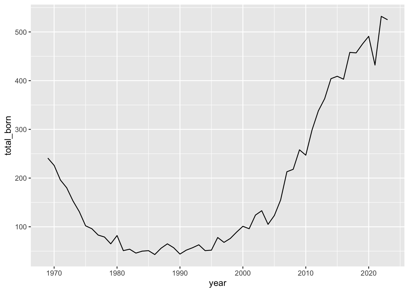
4.7 Classwork: Answering questions with group_by() and summarize()
Finally, use this data to answer the following questions:
- How many teenage births were there in Zürich between 2000 and 2020?
- What is the approximate age of oldest woman to ever give birth in each canton?
- How many children were born in Zurich, Bern and Geneva in 2019?
- How many children were born in each Canton in 1980?
- In each canton, what was the most common age range for mothers to give birth in 1970, 1990, and 2010?
4.8 Bonus questions
If you’ve finished all of these questions, here are some harder questions for more practice. I won’t go over these together with the class, but I’ll be happy to help you if you get stuck. The answers are also in the back of the book.
- Between 2010 and 2020, what were the average number of children born each year in each canton?
- Building off this, which years had an above average birth rate for that decade?
- Here’s some data about the number of deaths in each canton. https://opendata.swiss/de/dataset/todesfalle-nach-funf-jahres-altersgruppe-geschlecht-und-kanton-1969-2023 Can you download and clean this one?
- Simplify the births data into just number of births by year. Then join() this data with the deaths data. What was the total population change in Zürich in 2000? (Excluding immigration and emmigration)
- Make a plot of the total births and deaths in Basel-Stadt between 1970 and 2000.
4.9 Practice & Homework
So far, I’ve been giving you some functions to put into mutate() without much explanation. Your homework this week is to learn on your own what the following functions do. All of these are functions for working with strings of characters, and they’re very useful for cleaning data.
- str_count()
- str_to_upper()
- str_to_lower()
- str_to_title()
- str_sub()
- str_replace()
- str_replace_all()
- str_detect()
- str_length()
- str_to_sentence()
To experiment with these functions, you can try them out on a single string, for example:
## [1] 3If you have a dataset handy, you can also try them out on a column of a data frame. For example: