1 Getting Started
1.1 Why use R?
1.1.1 Reproducibility
Picture this: You’ve found an interesting data set, have downloaded the data, and have messed around manually making some plots in Excel. Months later, you want to make a similar plot for a different data set. You have to start from scratch, and try to remember every step you took. This is a horrible waste of time.
Instead, you could have written a script in R that would take the data set, clean it, and make the plot. You could then run this script on a new data set, and get the same plot.
Now picture this: You’ve done some advanced data analysis in SPSS, and you want to submit a paper to a journal. Reviewer 2 is especially strict, and wants to run the code you used to analyze the data. They don’t have SPSS, and end up rejecting your paper because they can’t verify your results. This is going to make your life very difficult.
Instead, if you use R, everything can be downloaded and set up for free. You can then share your code with the reviewer, and they can run it on their own computer.
1.1.2 Scalability
Many of the data sets we will use can be millions of lines of data, far too much to open in a spreadsheet program. R can handle these data sets with ease. It is also possible to preview your output on a small subset of your data, and then run it on the full data set, saving you time and resources.
1.1.3 Collaboration
Working in code makes it much easier to collaborate with other people on the same project. In this course, you will be able to share your code with others, and they will be able to run it on their own computers.
For the final project for this course, you will work in a small group to make a data visualization on a topic of your choice. More details about your final project will be available [here.][Final Presentations]
1.2 R vs Python
1.2.1 Python advantages
- Generally faster
- More popular outside of academia
- A much more consistent language, and the deeper parts of the language are easier to learn.
- Useful for things outside of data analysis & statistics. “The second best tool for any task.”
- Prettier, clearer syntax. You can pick up someone’s code and generally know exactly what it does. “A language for children and people with PhDs.”
1.2.2 R advantages:
- Statistics packages are more tightly curated.
- The Tidyverse is the best way to work with data.
- More flexible data visualization!
- Great publishing tools. This textbook was written entirely in Rstudio.
In the end, I encourage you to learn both someday. The two languages can really complement each other. For now, though, we will do everything in R.
1.3 Installation
Maybe the most difficult part of this course is getting everything set up. In our first lesson, all we’ll be doing is getting everything installed and set up. Let’s go!
1.3.1 Installing R & RStudio
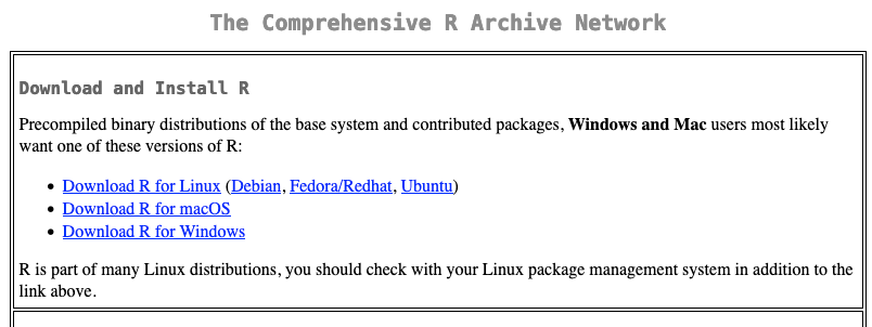
The exact steps you’ll take will vary depending on whether you’re using Mac, Windows or Linux, and whether you have a locked down university computer. Rather than list out every step you need to take, here are the general steps you’ll need to take to get started.
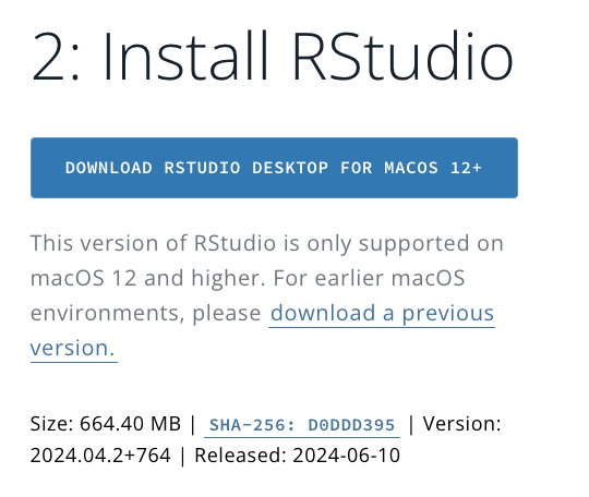
1.3.1.2 Install RStudio
Download RStudio from: - https://posit.co/download/rstudio-desktop/
Now open up RStudio, and you should see something like this:
![]()
Let’s make sure you have the right version of R installed. Find the window called “Console” in RStudio. By default, it is in the bottom left of the screen. Type the following into the console, and hit “Enter”.
## [1] "R version 4.4.1 (2024-06-14)"If you’ve done everything correctly, it will be 4.3 or 4.4.
1.3.2 Setting up RStudio
Before we start, let’s fiddle around with some settings. In the menu at the top of the screen, go to “Tools” > “Global Options”. Then open up the “Code” tab. Check the box that says “Use native pipe operator”
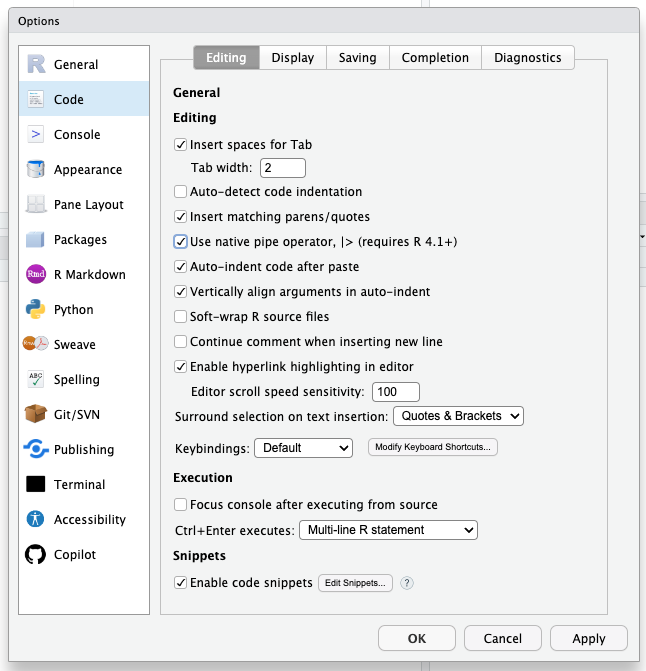
Don’t worry about what this means for now. You’ll know all about the pipe operator by the end of this course.
Next, go to the “Appearance” tab. You can change the theme of RStudio to something you like. I like “Tomorrow Night 80s”, but you can choose whatever you like.
While not directly covered in this course, also note the “Git” and “Copilot” tabs if you’re already familiar with them. These are very useful tools for working with code, and you should definitely check them out.
1.4 Setting up a Project
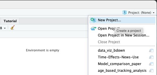
The first thing you should do when you start a new project is to create a new project in RStudio. This will keep all of your files and data in one place, and easy to find later.
To create a new project, go to “File” > “New Project”.
You should save it in a new directory (another word for folder).
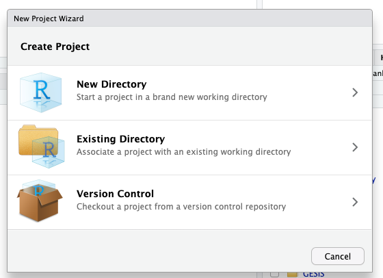
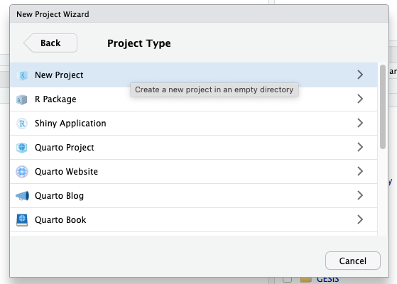
You’ll be presented with a list of options, but for this class I’d go with “New Project”.
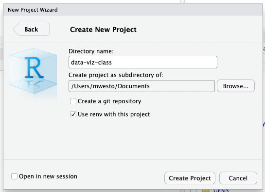
Finally, You can call it whatever you like and save it wherever you like, but I suggest something like “data_viz_class”, and maybe put it in your “Documents” folder.
1.5 R Basics
Finally! We’ve hit the end of the trust-me-and-just-do-it part of the course. Now we can start learning some R.
1.5.1 The world’s most over-engineered calculator.
As the first thing that we’ll do, let’s use R as a calculator to do some basic arithmetic. In the “Console” window, type the following:
## [1] 20You should see the number 20 appear in the console. You can also do most basic math the same way.
## [1] 31.41593Here, we can see that R knows what pi is, and can multiply it by 10. That’s because pi here is a variable, something that is saved in Rs memory, and can be used in calculations. We can make our own variables using the <- operator.
## [1] 78.53982Congratulations! You’ve just calculated the area of a circle with a radius of 5, using the formula A = pi * r^2.
You’ll also notice that in the upper right part of RStudio, there is a tab called “Environment”. This shows you all of the variables that you’ve created, and what their values are. You can also see the history of all the commands you’ve run in the “History” tab.
1.5.2 Actually writing code
The console is great for doing quick calculations, but you’ll start doing more complicated things soon, and you’ll want to save your work. Fortunately, we have tools for that. In this class, we’ll primarily be using scripts and notebooks. Scripts are just a list of commands that you want to run, and notebooks are a way to write text and code together.
To create a new script, go to “File” > “New File” > “R Script”.
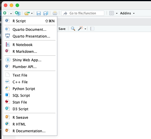
You can then write your code in the script, and save it as a normal file. Essentially, all computer code is just a text file that tells the computer what to do. You can run it by clicking the “Run” button in the upper right of the script window.
You’re writing your own code now, so mistakes happen and you can crash RStudio, or even your whole computer. Be sure to save your script as soon as you create it, and save it often.
This bears repeating, save your work.
Let’s save our script as week_1.R, in the main folder of your project. Now, look at the lower right window of RStudio. You should see a tab called “Files”. This is where you can see all of the files in your project. You can also create new folders and files here.
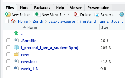
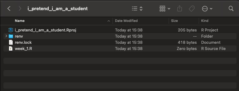
Just for good measure, go to your finder / file explorer/ file manager and find your project folder. You should see your new script there.
Let’s go back to RStudio, and type the following into your script:
## [1] "HUBERT"Now, start at the code you want to run, and press “Ctrl” + “Enter”. This will run the code in the console. You should see the word “HUBERT” appear in the console.
We can see a couple things from these two lines of code. First, we can see that we can save text in a variable, just like we can save numbers. Text in R is called a string.
Second, we can see that there’s a thing called toupper() that takes a string and makes it all uppercase. This is called a function. Functions are like little machines that take some input, do something to it, and then give you some output. You’ll learn a lot more about functions in this class. We can save the output of a function in a variable, just like we can save the output of a calculation.
## [1] "HUBERT"1.5.3 Installing Packages
The great thing about programming is that all the hard work is done for you already. If you want to do something, there is a 99% chance that someone has already written some code that does it for you. These pre-written bits of code are called packages. People write packages and freely share them with the world , and you can use them in your own code.
Let’s install a simple package! In the console (down below your script), type the following:
We can see that R is doing some work, and then it will tell you that the package has been installed. We do this in the console, not the script, because we only need to do this once. Once the package is installed, it will be available to you in all of your scripts.
This will install the package called “glue”. You can then use the functions in the package in your own code. To use the package, you need to load it into your R session. You can do this by typing the following into your script (up top):
Now, when you run your script, it will load the package, and you can use the functions in it. Let’s use the glue function to do something really basic, like glue two strings together. Add the following to your script:
## Hello, my name is Hubert!1.5.4 Installing the Tidyverse
For this class, we’ll be relying heavily on a package called the Tidyverse, short for “Tidy Universe”. It is, in my opinion, the one thing that makes R better than any other language for data analysis and visualization.
To install the Tidyverse, type the following into the console:
To make sure it installed correctly, add the following to your script:
Next week, we’ll start using the Tidyverse to do some basic data manipulation. Good job, you got everything up and running!
1.6 Practice & Homework
1.6.1 Practice 1: Typing
This is a very international class, and we all have slightly different keyboards. Your first assignment is to figure out how to type the following keys on your keyboard:
& $ | [] {} () \ / ~ ` ^ < > %1.6.2 Practice 2: Getting familiar with R.
This week, I just want you to get a little more familiar with R. The following mini-course, which can be done entirely in RStudio, will walk you through some of the basics of the language.
To start, install the Swirl package by typing the following into the console:
Then, type the following into the console:
This will create a little interactive course that you can do in RStudio. For your homework, try your hardest to work through lessons 1-9. Don’t worry too much about memorizing every single thing, we will get better through practice.