Week 2
# This is all copied from the "Import Data" dialog.
cows <- read_delim("input_data/cattle-NamesFemaleCalves.csv",
    delim = ";", escape_double = FALSE, trim_ws = TRUE,
    skip = 1)
## Rows: 592 Columns: 5
## ── Column specification ─────────────────────────────────────────────────────────────────────────────────────────────────────────────────────────────────────────────────────────────────────────────────────────────────────────────────────────────────────────────────────
## Delimiter: ";"
## chr (2): Name, OwnerLanguage
## dbl (3): count, Rank, year
##
## ℹ Use `spec()` to retrieve the full column specification for this data.
## ℹ Specify the column types or set `show_col_types = FALSE` to quiet this message.
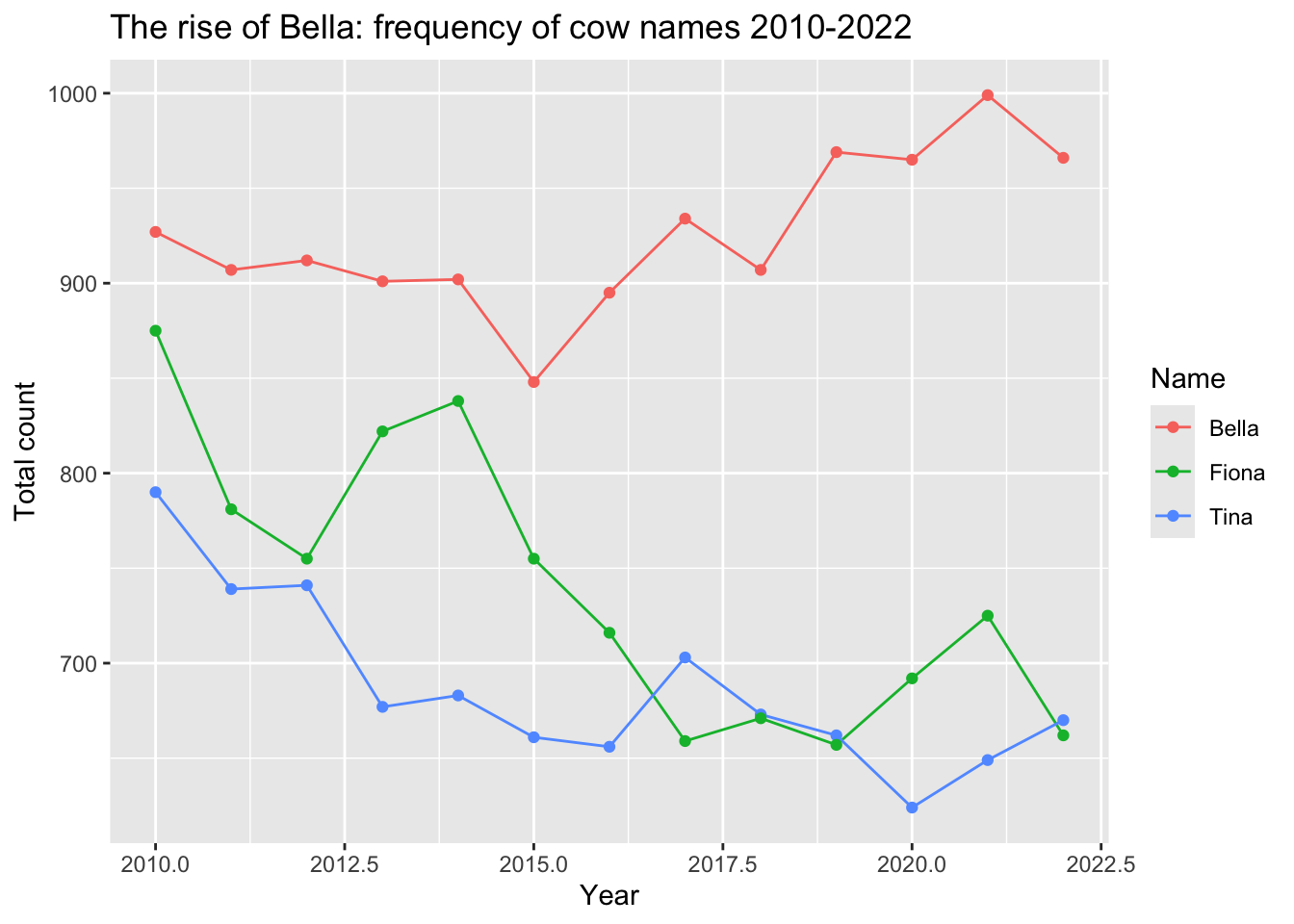
cows |>
  # I only want these three names
  filter(Name %in% c("Bella", "Fiona", "Tina")) |>

  # This contains separate data for each language,
  # but I just want the "all" data.
  filter(OwnerLanguage == "__all__") |>

  # I only want the data for the years before 2023
  filter(year < 2023) |>

  # I only want the columns Name, count, and year
  select(Name, count, year) |>

  # Now we put everything into ggplot!
  # We add aesthetics (aes) to tell ggplot which columns
  # to use for x and y, and the color
  ggplot(aes(x=year, y=count, color=Name)) +

  # We add a line and points
  geom_line() +
  geom_point() +

  # We add a title and labels
  labs(
    title="The rise of Bella: frequency of cow names 2010-2022",
    x = "Year",
    y= "Total count"
  )
Week 4 Bonus Questions
- Between 2010 and 2020, what were the average number of children born each year in each canton?
births |>
  filter(year >= 2010, year <= 2020) |>
  group_by(canton_name, year) |>
  summarise(total_births_per_year = sum(total_born)) |>
  summarize(avg_born = mean(total_births_per_year))
## # A tibble: 26 × 2
##    canton_name            avg_born
##    <chr>                     <dbl>
##  1 Aargau                    6682.
##  2 Appenzell Ausserrhoden     545.
##  3 Appenzell Innerrhoden      175.
##  4 Basel-Landschaft          2532.
##  5 Basel-Stadt               1983.
##  6 Bern                      9820.
##  7 Freiburg                  3332.
##  8 Genf                      5229
##  9 Glarus                     382.
## 10 Graubünden                1715
## # ℹ 16 more rows
- Building off this, which years had an above average birth rate for that decade?
births |>
  filter(year >= 2010, year <= 2020) |>
  group_by(canton_name, year) |>
  summarise(total_births_per_year = sum(total_born)) |>
  summarize(year = year, total_births_per_year = total_births_per_year, avg_born = mean(total_births_per_year)) |>
  mutate(above_average = total_births_per_year > avg_born) |>
  filter(above_average) |>
  select(canton_name, year)
## # A tibble: 154 × 2
## # Groups:   canton_name [26]
##    canton_name             year
##    <chr>                  <dbl>
##  1 Aargau                  2014
##  2 Aargau                  2015
##  3 Aargau                  2016
##  4 Aargau                  2017
##  5 Aargau                  2018
##  6 Aargau                  2019
##  7 Aargau                  2020
##  8 Appenzell Ausserrhoden  2015
##  9 Appenzell Ausserrhoden  2016
## 10 Appenzell Ausserrhoden  2017
## # ℹ 144 more rows
- Here’s some data about the number of deaths in each canton. https://opendata.swiss/de/dataset/todesfalle-nach-funf-jahres-altersgruppe-geschlecht-und-kanton-1969-2023 Can you download and clean this one?
download.file("https://dam-api.bfs.admin.ch/hub/api/dam/assets/32007751/master", "input_data/deaths.csv")
deaths <- read_csv("input_data/deaths.csv")
## Rows: 89100 Columns: 5
## ── Column specification ─────────────────────────────────────────────────────────────────────────────────────────────────────────────────────────────────────────────────────────────────────────────────────────────────────────────────────────────────────────────────────
## Delimiter: ","
## chr (3): CANTON, AGE, SEX
## dbl (2): YEAR, OBS_VALUE
##
## ℹ Use `spec()` to retrieve the full column specification for this data.
## ℹ Specify the column types or set `show_col_types = FALSE` to quiet this message.
colnames(deaths) <- c("year", "canton", "age", "sex", "total_deaths")


deaths <- deaths |>
  filter(age == "_T") |>
  filter(canton != "CH") |>
  filter(sex == "T") |>
  select(-age, -sex)

deaths
## # A tibble: 1,430 × 3
##     year canton total_deaths
##    <dbl> <chr>         <dbl>
##  1  1969 1              9846
##  2  1969 2              8836
##  3  1969 3              2405
##  4  1969 4               283
##  5  1969 5               830
##  6  1969 6               231
##  7  1969 7               201
##  8  1969 8               431
##  9  1969 9               526
## 10  1969 10             1728
## # ℹ 1,420 more rows
- Simplify the births data into just number of births by year. Then join this data with the deaths data. What was the total population change in each canton?
births <- births |>
  group_by(year, canton_number, canton_name) |>
  summarize(total_births = sum(total_born))

births
## # A tibble: 1,430 × 4
## # Groups:   year, canton_number [1,430]
##     year canton_number canton_name            total_births
##    <dbl> <chr>         <chr>                         <dbl>
##  1  1969 1             Zürich                        16638
##  2  1969 10            Freiburg                       3187
##  3  1969 11            Solothurn                      3759
##  4  1969 12            Basel-Stadt                    2833
##  5  1969 13            Basel-Landschaft               3958
##  6  1969 14            Schaffhausen                   1170
##  7  1969 15            Appenzell Ausserrhoden          774
##  8  1969 16            Appenzell Innerrhoden           274
##  9  1969 17            St. Gallen                     7229
## 10  1969 18            Graubünden                     2819
## # ℹ 1,420 more rows
deaths <- deaths |>
  rename(canton_number = canton)

birth_and_deaths <- births |>
  left_join(deaths)
## Joining with `by = join_by(year, canton_number)`
## # A tibble: 1,430 × 5
## # Groups:   year, canton_number [1,430]
##     year canton_number canton_name            total_births total_deaths
##    <dbl> <chr>         <chr>                         <dbl>        <dbl>
##  1  1969 1             Zürich                        16638         9846
##  2  1969 10            Freiburg                       3187         1728
##  3  1969 11            Solothurn                      3759         1907
##  4  1969 12            Basel-Stadt                    2833         2398
##  5  1969 13            Basel-Landschaft               3958         1491
##  6  1969 14            Schaffhausen                   1170          755
##  7  1969 15            Appenzell Ausserrhoden          774          656
##  8  1969 16            Appenzell Innerrhoden           274          192
##  9  1969 17            St. Gallen                     7229         3726
## 10  1969 18            Graubünden                     2819         1570
## # ℹ 1,420 more rows
birth_and_deaths <- birth_and_deaths |>
  mutate(total_population_change = total_births - total_deaths)

birth_and_deaths
## # A tibble: 1,430 × 6
## # Groups:   year, canton_number [1,430]
##     year canton_number canton_name            total_births total_deaths total_population_change
##    <dbl> <chr>         <chr>                         <dbl>        <dbl>                   <dbl>
##  1  1969 1             Zürich                        16638         9846                    6792
##  2  1969 10            Freiburg                       3187         1728                    1459
##  3  1969 11            Solothurn                      3759         1907                    1852
##  4  1969 12            Basel-Stadt                    2833         2398                     435
##  5  1969 13            Basel-Landschaft               3958         1491                    2467
##  6  1969 14            Schaffhausen                   1170          755                     415
##  7  1969 15            Appenzell Ausserrhoden          774          656                     118
##  8  1969 16            Appenzell Innerrhoden           274          192                      82
##  9  1969 17            St. Gallen                     7229         3726                    3503
## 10  1969 18            Graubünden                     2819         1570                    1249
## # ℹ 1,420 more rows
birth_and_deaths |>
  filter(year == 2000) |>
  filter(canton_name == "Zürich") |>
  select(total_population_change)
## Adding missing grouping variables: `year`, `canton_number`
## # A tibble: 1 × 3
## # Groups:   year, canton_number [1]
##    year canton_number total_population_change
##   <dbl> <chr>                           <dbl>
## 1  2000 1                                2485
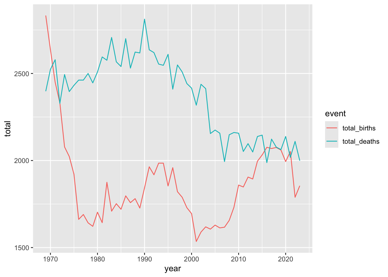
- Make a plot of the total births and deaths in Basel-Stadt between 1970 and 2000.
birth_and_deaths |>
  filter(canton_name == "Basel-Stadt") |>
  select(year, canton_name, total_births, total_deaths) |>
  pivot_longer(cols = c(total_births, total_deaths), names_to = "event", values_to = "total") |>
  ggplot(aes(x = year, y = total, color = event)) +
  geom_line()
## Adding missing grouping variables: `canton_number`