13 Tables and Statistics
For this class, we’ll be using some new packages, gt, gtsummary, and broom. Install and load them before we begin.
install.packages("gt")
install.packages("gtsummary")
install.packages("broom")
install.packages("broom.helpers")
install.packages("webshot2")library(gt)
library(gtsummary)
library(broom)
library(tidyverse)
library(gapminder) # Interesting data set about life expectancy, population, gdp, etc.
library(sf)13.1 Making nice tables
Sometimes, our visualizations just won’t cut it, and we need to just make a table out of the data. To start out, we’ll once again use the gapminder data set.
## Rows: 1,704
## Columns: 6
## $ country   <fct> "Afghanistan", "Afghanistan", "Afghanistan", "Afghanistan", "Afghanistan", "Afghanistan", "Afghanistan", "Afghanistan", "Afghanistan", "Afghanistan", "Afghanistan", "Afghanistan", "Albania", "Albania", "Albania", "Albania", "Albania", "Albania", "Al…
## $ continent <fct> Asia, Asia, Asia, Asia, Asia, Asia, Asia, Asia, Asia, Asia, Asia, Asia, Europe, Europe, Europe, Europe, Europe, Europe, Europe, Europe, Europe, Europe, Europe, Europe, Africa, Africa, Africa, Africa, Africa, Africa, Africa, Africa, Africa, Africa, A…
## $ year      <int> 1952, 1957, 1962, 1967, 1972, 1977, 1982, 1987, 1992, 1997, 2002, 2007, 1952, 1957, 1962, 1967, 1972, 1977, 1982, 1987, 1992, 1997, 2002, 2007, 1952, 1957, 1962, 1967, 1972, 1977, 1982, 1987, 1992, 1997, 2002, 2007, 1952, 1957, 1962, 1967, 1972, 197…
## $ lifeExp   <dbl> 28.801, 30.332, 31.997, 34.020, 36.088, 38.438, 39.854, 40.822, 41.674, 41.763, 42.129, 43.828, 55.230, 59.280, 64.820, 66.220, 67.690, 68.930, 70.420, 72.000, 71.581, 72.950, 75.651, 76.423, 43.077, 45.685, 48.303, 51.407, 54.518, 58.014, 61.368, 6…
## $ pop       <int> 8425333, 9240934, 10267083, 11537966, 13079460, 14880372, 12881816, 13867957, 16317921, 22227415, 25268405, 31889923, 1282697, 1476505, 1728137, 1984060, 2263554, 2509048, 2780097, 3075321, 3326498, 3428038, 3508512, 3600523, 9279525, 10270856, 1100…
## $ gdpPercap <dbl> 779.4453, 820.8530, 853.1007, 836.1971, 739.9811, 786.1134, 978.0114, 852.3959, 649.3414, 635.3414, 726.7341, 974.5803, 1601.0561, 1942.2842, 2312.8890, 2760.1969, 3313.4222, 3533.0039, 3630.8807, 3738.9327, 2497.4379, 3193.0546, 4604.2117, 5937.029…
To make a table, simply use the gt() function. This creates a tidy looking table that we’ll be able to export.
For our purposes, though, we’ll want to filter the data to only show Mongolia, so that our table will fit on a single page.
| country | continent | year | lifeExp | pop | gdpPercap |
|---|---|---|---|---|---|
| Mongolia | Asia | 1952 | 42.244 | 800663 | 786.5669 |
| Mongolia | Asia | 1957 | 45.248 | 882134 | 912.6626 |
| Mongolia | Asia | 1962 | 48.251 | 1010280 | 1056.3540 |
| Mongolia | Asia | 1967 | 51.253 | 1149500 | 1226.0411 |
| Mongolia | Asia | 1972 | 53.754 | 1320500 | 1421.7420 |
| Mongolia | Asia | 1977 | 55.491 | 1528000 | 1647.5117 |
| Mongolia | Asia | 1982 | 57.489 | 1756032 | 2000.6031 |
| Mongolia | Asia | 1987 | 60.222 | 2015133 | 2338.0083 |
| Mongolia | Asia | 1992 | 61.271 | 2312802 | 1785.4020 |
| Mongolia | Asia | 1997 | 63.625 | 2494803 | 1902.2521 |
| Mongolia | Asia | 2002 | 65.033 | 2674234 | 2140.7393 |
| Mongolia | Asia | 2007 | 66.803 | 2874127 | 3095.7723 |
13.2 Exporting tables
Similarly to ggsave(), we can use gtsave() to save our tables to a file. We can save them as a Word document, an HTML file, or a PNG image. This is going to make it easy to share with your collaborators and include in your reports.
13.3 Classwork: Export a table
- Use some filtering, grouping, and summarizing to create a table that shows the average life expectancy by country in Europe.
- Export this table to a Word document.
13.4 Summary statistics
Traditionally, a scientific paper will have two tables: one for the descriptive statistics and one for the regression results. The descriptive statistics table will show the mean, median, and standard deviation for continuous variables, and the count and percentage for categorical variables. The tbl_summary() function from the gtsummary package will do this for us automatically.
| Characteristic | N = 1,7041 |
|---|---|
| continent | |
| Africa | 624 (37%) |
| Americas | 300 (18%) |
| Asia | 396 (23%) |
| Europe | 360 (21%) |
| Oceania | 24 (1.4%) |
| year | 1,980 (1,965, 1,995) |
| lifeExp | 61 (48, 71) |
| pop | 7,023,596 (2,792,776, 19,593,661) |
| gdpPercap | 3,532 (1,202, 9,326) |
| 1 n (%); Median (Q1, Q3) | |
There are a lot of options that we can change in the tbl_summary() function. For example, we can change the type of variable, the label, the number of digits to round to, and the statistics to show.
Here, we’ll change the type of the year variable to categorical, change the label of the year variable, round the lifeExp variable to two digits, and change the statistics to show for continuous and categorical variables.
Gt is a very new package, so the way things work changes all the time. Don’t put too much brain power into memorizing this stuff, and just read the docs here:
gapminder |>
  select(-country) |>
  tbl_summary(
    type = list(year ~ "categorical"), # Change between continuous and categorical
    label = list(year ~ "Year"), # Change the label without having to rename the column
    digits = list(lifeExp ~ 2, pop ~ 0), # Change the number of digits to round to
    statistic = list(
      all_continuous() ~ c("{min}, {mean}, {max}"), # Change the statistics to show for continuous variables
      all_categorical() ~ "{n} / {N} ({p}%)" # Change the statistics to show for categorical variables
    ),
)| Characteristic | N = 1,7041 |
|---|---|
| continent | |
| Africa | 624 / 1,704 (37%) |
| Americas | 300 / 1,704 (18%) |
| Asia | 396 / 1,704 (23%) |
| Europe | 360 / 1,704 (21%) |
| Oceania | 24 / 1,704 (1.4%) |
| Year | |
| 1952 | 142 / 1,704 (8.3%) |
| 1957 | 142 / 1,704 (8.3%) |
| 1962 | 142 / 1,704 (8.3%) |
| 1967 | 142 / 1,704 (8.3%) |
| 1972 | 142 / 1,704 (8.3%) |
| 1977 | 142 / 1,704 (8.3%) |
| 1982 | 142 / 1,704 (8.3%) |
| 1987 | 142 / 1,704 (8.3%) |
| 1992 | 142 / 1,704 (8.3%) |
| 1997 | 142 / 1,704 (8.3%) |
| 2002 | 142 / 1,704 (8.3%) |
| 2007 | 142 / 1,704 (8.3%) |
| lifeExp | 23.60, 59.47, 82.60 |
| pop | 60,011, 29,601,212, 1,318,683,096 |
| gdpPercap | 241, 7,215, 113,523 |
| 1 n / N (%); Min, Mean, Max | |
13.5 How to read a regression model
Next, in a scientific paper, we often run a regression model to see how different variables are related to each other. The lm() function in R will run a linear regression model for us. We can then use the summary() function to see the results.
Here, I’m looking at the effect of the year on life expectancy. The lm() function takes the formula y ~ x, where y is the dependent variable and x is the independent variable. The summary() function will show us the results of the regression model.
##
## Call:
## lm(formula = lifeExp ~ year, data = gapminder)
##
## Residuals:
##     Min      1Q  Median      3Q     Max
## -39.949  -9.651   1.697  10.335  22.158
##
## Coefficients:
##               Estimate Std. Error t value            Pr(>|t|)
## (Intercept) -585.65219   32.31396  -18.12 <0.0000000000000002 ***
## year           0.32590    0.01632   19.96 <0.0000000000000002 ***
## ---
## Signif. codes:  0 '***' 0.001 '**' 0.01 '*' 0.05 '.' 0.1 ' ' 1
##
## Residual standard error: 11.63 on 1702 degrees of freedom
## Multiple R-squared:  0.1898, Adjusted R-squared:  0.1893
## F-statistic: 398.6 on 1 and 1702 DF,  p-value: < 0.00000000000000022
But what does this mean? The Estimate column shows the effect of the independent variable on the dependent variable. In this case, the year variable has a coefficient of 0.325, which means that for every year, the life expectancy increases by 0.325 years. The Pr(>|t|) column shows the p-value of the coefficient. In this case, the p-value is less than 0.05, which means that the effect of the year on life expectancy is statistically significant. R-squared is a measure of how well the model fits the data. It ranges from 0 to 1, with 1 being a perfect fit. In this case, the R-squared is 0.1898, which means that the year explains 19% of the variation in life expectancy.
You can include multiple regressors, separated by a +, and this will condition on the other variables. Here, we condition on each continent, which is a categorical variable.
##
## Call:
## lm(formula = lifeExp ~ year + continent, data = gapminder)
##
## Residuals:
##      Min       1Q   Median       3Q      Max
## -29.3401  -4.3842   0.1598   4.5875  20.6759
##
## Coefficients:
##                     Estimate Std. Error t value            Pr(>|t|)
## (Intercept)       -596.26130   20.32816  -29.33 <0.0000000000000002 ***
## year                 0.32590    0.01027   31.74 <0.0000000000000002 ***
## continentAmericas   15.79341    0.51400   30.73 <0.0000000000000002 ***
## continentAsia       11.19957    0.47005   23.83 <0.0000000000000002 ***
## continentEurope     23.03836    0.48421   47.58 <0.0000000000000002 ***
## continentOceania    25.46088    1.52184   16.73 <0.0000000000000002 ***
## ---
## Signif. codes:  0 '***' 0.001 '**' 0.01 '*' 0.05 '.' 0.1 ' ' 1
##
## Residual standard error: 7.316 on 1698 degrees of freedom
## Multiple R-squared:  0.6801, Adjusted R-squared:  0.6792
## F-statistic: 722.1 on 5 and 1698 DF,  p-value: < 0.00000000000000022
Take a statistics class to learn more about this.
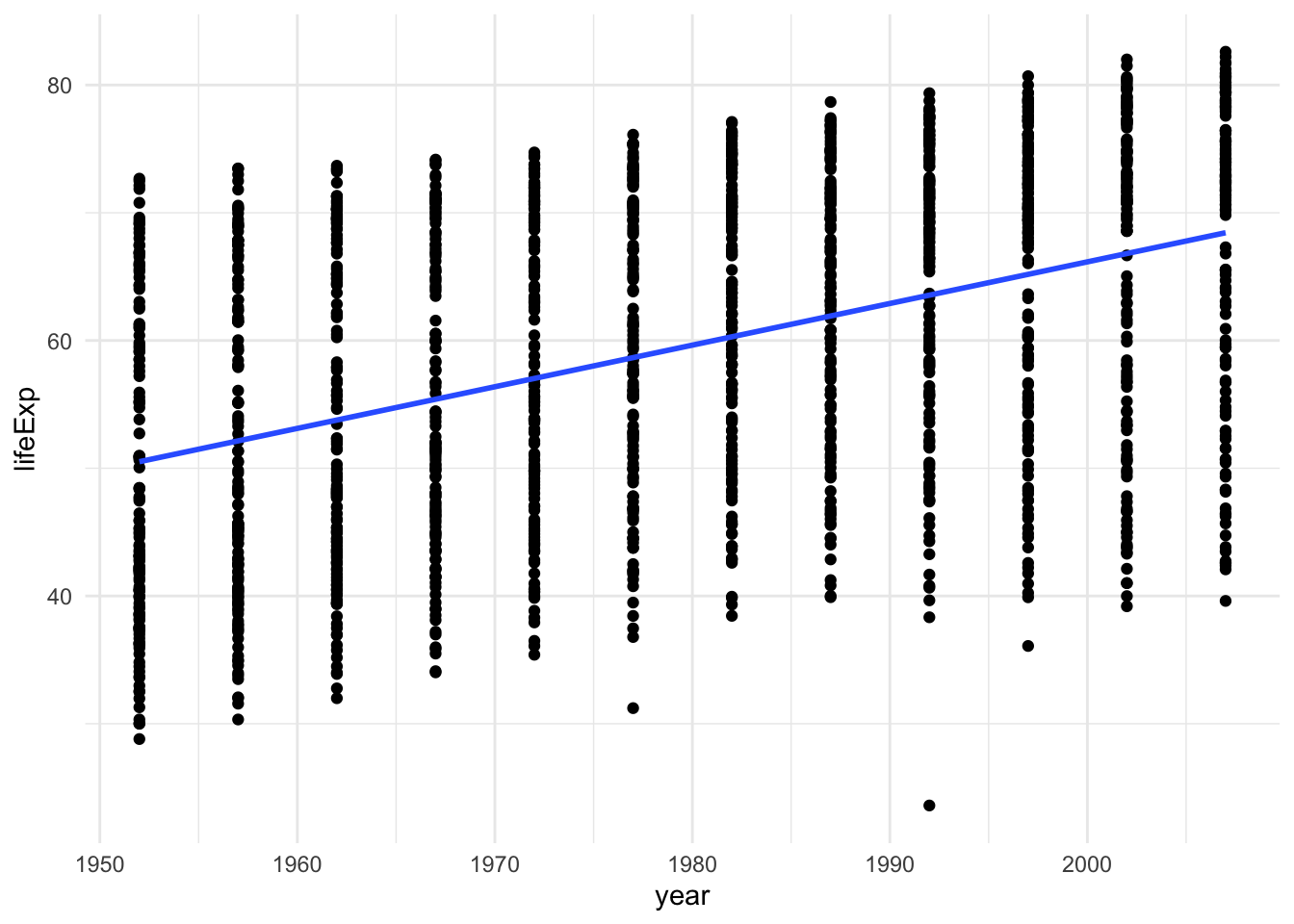
Remember back when we did some geom_smooth() stuff? the method argument can be set to "lm" to show the regression line. This is a quick and dirty way to show the regression line on a scatter plot.
gapminder |> ggplot(aes(x = year, y = lifeExp)) +
  geom_point() +
  geom_smooth(method = "lm", se = FALSE) +
  theme_minimal()
## `geom_smooth()` using formula = 'y ~ x'
These regression tables can be exported as well, using the tbl_regression() function from the gtsummary package.
| Characteristic | Beta | 95% CI1 | p-value |
|---|---|---|---|
| year | 0.33 | 0.31, 0.35 | <0.001 |
| continent | |||
| Africa | — | — | |
| Americas | 16 | 15, 17 | <0.001 |
| Asia | 11 | 10, 12 | <0.001 |
| Europe | 23 | 22, 24 | <0.001 |
| Oceania | 25 | 22, 28 | <0.001 |
| 1 CI = Confidence Interval | |||
To save it, you have to first convert it to a gt table using the as_gt() function, and then use the gtsave() function to save it to a file.
13.6 Classwork: Do a whole scientific study
For our final classwork, you’re going to be a social scientist, and find the relationship between some statistics about European countries. You’ll need to find some data, clean it, and run a regression model to see how different variables are related to each other. You’ll then need to make a table of the descriptive statistics and a table of the regression results.
This will bring together stuff we’ve learned throughout the course, so you’ll want to also look back at the previous lessons.
- First, load some data about a continent of your choice.
- Now, think of two things that might be related to each other. For example, you could look at the relationship between health spending and life expectancy. Use the
wbsearch()function to find the indicators that you need.
- Next, load and clean the data, as we did before.
health_expenditure <- wb_data(indicator = "SH.XPD.CHEX.GD.ZS", start_date = 2020, end_date = 2020)
health_expenditure <- health_expenditure |> rename(spending = SH.XPD.CHEX.GD.ZS)
health_expenditure |> glimpse()
## Rows: 217
## Columns: 9
## $ iso2c <chr> "AW", "AF", "AO", "AL", "AD", "AE", "AR", "AM", "AS", "AG", "AU", "AT", "AZ", "BI", "BE", "BJ", "BF", "BD", "BG", "BH", "BS", "BA", "BY", "BZ", "BM", "BO", "BR", "BB", "BN", "BT", "BW", "CF", "CA", "CH", "JG", "CL", "CN", "CI", "CM", "CD", "CG", …
## $ iso3c <chr> "ABW", "AFG", "AGO", "ALB", "AND", "ARE", "ARG", "ARM", "ASM", "ATG", "AUS", "AUT", "AZE", "BDI", "BEL", "BEN", "BFA", "BGD", "BGR", "BHR", "BHS", "BIH", "BLR", "BLZ", "BMU", "BOL", "BRA", "BRB", "BRN", "BTN", "BWA", "CAF", "CAN", "CHE", "CHI", "…
## $ country <chr> "Aruba", "Afghanistan", "Angola", "Albania", "Andorra", "United Arab Emirates", "Argentina", "Armenia", "American Samoa", "Antigua and Barbuda", "Australia", "Austria", "Azerbaijan", "Burundi", "Belgium", "Benin", "Burkina Faso", "Bangladesh", "B…
## $ date <dbl> 2020, 2020, 2020, 2020, 2020, 2020, 2020, 2020, 2020, 2020, 2020, 2020, 2020, 2020, 2020, 2020, 2020, 2020, 2020, 2020, 2020, 2020, 2020, 2020, 2020, 2020, 2020, 2020, 2020, 2020, 2020, 2020, 2020, 2020, 2020, 2020, 2020, 2020, 2020, 2020, 2020, …
## $ spending <dbl> NA, 15.533614, 3.220706, 7.519203, 8.786739, 5.824770, 10.347015, 12.240000, NA, 5.921462, 10.683737, 11.390000, 5.850000, 10.718372, 11.197513, 2.469704, 6.501933, 2.270639, 8.480000, 4.716848, 7.647008, 9.700000, 6.410000, 5.309744, NA, 8.02258…
## $ unit <chr> NA, NA, NA, NA, NA, NA, NA, NA, NA, NA, NA, NA, NA, NA, NA, NA, NA, NA, NA, NA, NA, NA, NA, NA, NA, NA, NA, NA, NA, NA, NA, NA, NA, NA, NA, NA, NA, NA, NA, NA, NA, NA, NA, NA, NA, NA, NA, NA, NA, NA, NA, NA, NA, NA, NA, NA, NA, NA, NA, NA, NA, NA…
## $ obs_status <chr> NA, NA, NA, NA, NA, NA, NA, NA, NA, NA, NA, NA, NA, NA, NA, NA, NA, NA, NA, NA, NA, NA, NA, NA, NA, NA, NA, NA, NA, NA, NA, NA, NA, NA, NA, NA, NA, NA, NA, NA, NA, NA, NA, NA, NA, NA, NA, NA, NA, NA, NA, NA, NA, NA, NA, NA, NA, NA, NA, NA, NA, NA…
## $ footnote <chr> NA, NA, NA, NA, NA, NA, NA, NA, NA, NA, NA, NA, NA, NA, NA, NA, NA, NA, NA, NA, NA, NA, NA, NA, NA, NA, NA, NA, NA, NA, NA, NA, NA, NA, NA, NA, NA, NA, NA, NA, NA, NA, NA, NA, NA, NA, NA, NA, NA, NA, NA, NA, NA, NA, NA, NA, NA, NA, NA, NA, NA, NA…
## $ last_updated <date> 2024-11-13, 2024-11-13, 2024-11-13, 2024-11-13, 2024-11-13, 2024-11-13, 2024-11-13, 2024-11-13, 2024-11-13, 2024-11-13, 2024-11-13, 2024-11-13, 2024-11-13, 2024-11-13, 2024-11-13, 2024-11-13, 2024-11-13, 2024-11-13, 2024-11-13, 2024-11-13, 2024-…life_expectancy <- wb_data(indicator = "SP.DYN.LE00.IN", start_date = 2020, end_date = 2020)
life_expectancy <- life_expectancy |> rename(years_to_live = SP.DYN.LE00.IN)
life_expectancy |> glimpse()## Rows: 217
## Columns: 9
## $ iso2c <chr> "AW", "AF", "AO", "AL", "AD", "AE", "AR", "AM", "AS", "AG", "AU", "AT", "AZ", "BI", "BE", "BJ", "BF", "BD", "BG", "BH", "BS", "BA", "BY", "BZ", "BM", "BO", "BR", "BB", "BN", "BT", "BW", "CF", "CA", "CH", "JG", "CL", "CN", "CI", "CM", "CD", "CG",…
## $ iso3c <chr> "ABW", "AFG", "AGO", "ALB", "AND", "ARE", "ARG", "ARM", "ASM", "ATG", "AUS", "AUT", "AZE", "BDI", "BEL", "BEN", "BFA", "BGD", "BGR", "BHR", "BHS", "BIH", "BLR", "BLZ", "BMU", "BOL", "BRA", "BRB", "BRN", "BTN", "BWA", "CAF", "CAN", "CHE", "CHI", …
## $ country <chr> "Aruba", "Afghanistan", "Angola", "Albania", "Andorra", "United Arab Emirates", "Argentina", "Armenia", "American Samoa", "Antigua and Barbuda", "Australia", "Austria", "Azerbaijan", "Burundi", "Belgium", "Benin", "Burkina Faso", "Bangladesh", "…
## $ date <dbl> 2020, 2020, 2020, 2020, 2020, 2020, 2020, 2020, 2020, 2020, 2020, 2020, 2020, 2020, 2020, 2020, 2020, 2020, 2020, 2020, 2020, 2020, 2020, 2020, 2020, 2020, 2020, 2020, 2020, 2020, 2020, 2020, 2020, 2020, 2020, 2020, 2020, 2020, 2020, 2020, 2020,…
## $ years_to_live <dbl> 75.72300, 62.57500, 62.26100, 76.98900, NA, 78.94600, 75.89200, 72.17300, NA, 78.84100, 83.20000, 81.19268, 66.86800, 61.56600, 80.69512, 60.08800, 59.73100, 71.96800, 73.65854, 79.17400, 72.67700, 76.22500, 72.45722, 72.85400, 81.13600, 64.4670…
## $ unit <chr> NA, NA, NA, NA, NA, NA, NA, NA, NA, NA, NA, NA, NA, NA, NA, NA, NA, NA, NA, NA, NA, NA, NA, NA, NA, NA, NA, NA, NA, NA, NA, NA, NA, NA, NA, NA, NA, NA, NA, NA, NA, NA, NA, NA, NA, NA, NA, NA, NA, NA, NA, NA, NA, NA, NA, NA, NA, NA, NA, NA, NA, N…
## $ obs_status <chr> NA, NA, NA, NA, NA, NA, NA, NA, NA, NA, NA, NA, NA, NA, NA, NA, NA, NA, NA, NA, NA, NA, NA, NA, NA, NA, NA, NA, NA, NA, NA, NA, NA, NA, NA, NA, NA, NA, NA, NA, NA, NA, NA, NA, NA, NA, NA, NA, NA, NA, NA, NA, NA, NA, NA, NA, NA, NA, NA, NA, NA, N…
## $ footnote <chr> NA, NA, NA, NA, NA, NA, NA, NA, NA, NA, NA, NA, NA, NA, NA, NA, NA, NA, NA, NA, NA, NA, NA, NA, NA, NA, NA, NA, NA, NA, NA, NA, NA, NA, NA, NA, NA, NA, NA, NA, NA, NA, NA, NA, NA, NA, NA, NA, NA, NA, NA, NA, NA, NA, NA, NA, NA, NA, NA, NA, NA, N…
## $ last_updated <date> 2024-11-13, 2024-11-13, 2024-11-13, 2024-11-13, 2024-11-13, 2024-11-13, 2024-11-13, 2024-11-13, 2024-11-13, 2024-11-13, 2024-11-13, 2024-11-13, 2024-11-13, 2024-11-13, 2024-11-13, 2024-11-13, 2024-11-13, 2024-11-13, 2024-11-13, 2024-11-13, 2024…- Now, join the data together and save it as a new data frame.
europe_data <- europe |>
  left_join(health_expenditure, by = c("iso_a3" = "iso3c")) |>
left_join(life_expectancy, by = c("iso_a3" = "iso3c"))- Now, make a table of the descriptive statistics.
| Country | Current health expenditure (% of GDP) | Life expectancy at birth, total (years) |
|---|---|---|
| Albania | 7.519203 | 76.98900 |
| Austria | 11.390000 | 81.19268 |
| Belarus | 6.410000 | 72.45722 |
| Belgium | 11.197513 | 80.69512 |
| Bosnia and Herz. | 9.700000 | 76.22500 |
| Bulgaria | 8.480000 | 73.65854 |
| Croatia | 7.720000 | 77.72439 |
| Czechia | 9.213688 | 78.17561 |
| Denmark | 10.560000 | 81.60244 |
| Estonia | 7.579065 | 78.59512 |
| Finland | 9.630000 | 81.93171 |
| France | NA | NA |
| Germany | 12.692553 | 81.04146 |
| Greece | 9.503638 | 81.28780 |
| Hungary | 7.290000 | 75.56829 |
| Iceland | 9.610000 | 83.06341 |
| Ireland | 7.109147 | 82.55610 |
| Italy | 9.630000 | 82.19512 |
| Kosovo | NA | NA |
| Latvia | 7.250000 | 75.18537 |
| Lithuania | 7.480000 | 74.97805 |
| Luxembourg | 5.740000 | 82.14390 |
| Moldova | 7.000000 | 70.16600 |
| Montenegro | 11.420000 | 75.93171 |
| Netherlands | 11.210000 | 81.35854 |
| North Macedonia | 7.730000 | 74.39512 |
| Norway | NA | NA |
| Poland | 6.500000 | 76.50000 |
| Portugal | 10.550000 | 80.97561 |
| Romania | 6.230000 | 74.25366 |
| Russia | 7.570000 | 71.33878 |
| Serbia | 8.700421 | 74.47805 |
| Slovakia | 7.130000 | 76.86585 |
| Slovenia | 9.430000 | 80.53171 |
| Spain | 10.745660 | 82.33171 |
| Sweden | 11.330000 | 82.35610 |
| Switzerland | 11.732068 | 83.00000 |
| Ukraine | 7.560000 | 71.18512 |
| United Kingdom | 12.158634 | 80.35122 |
- This is probably too much information, so let’s just do a table of the basic summary statistics.
| Characteristic | N = 391 |
|---|---|
| GDP (in million USD) | 209,852 (51,475, 533,097) |
| Current health expenditure (% of GDP) | 8.96 (7.39, 10.65) |
| Unknown | 3 |
| Life expectancy at birth, total (years) | 78.4 (75.1, 81.5) |
| Unknown | 3 |
| 1 Median (Q1, Q3) | |
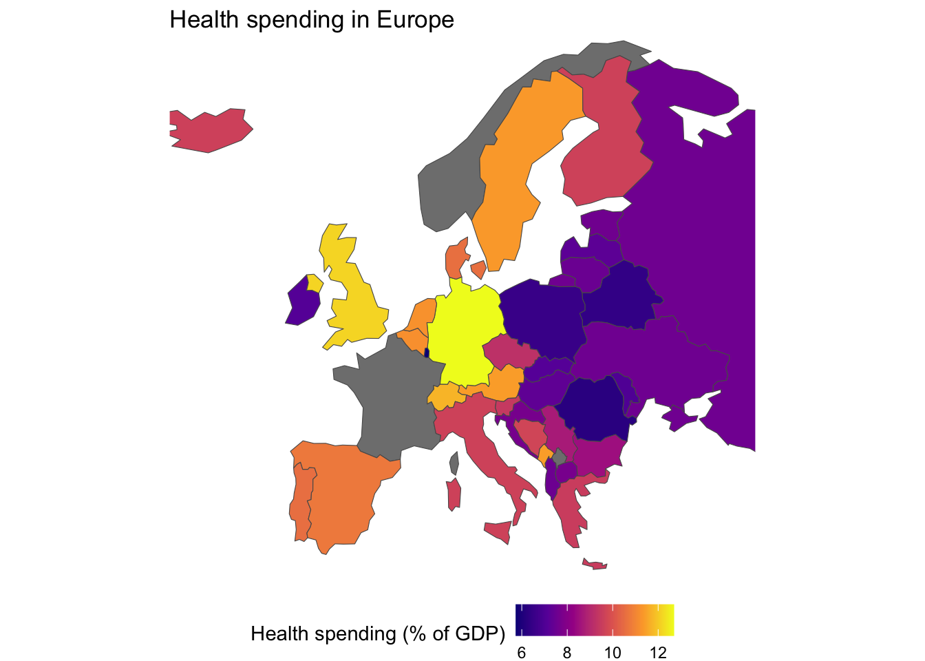
- If you want, make a map of the data. We’ve done enough of this, so you can skip it if you like.

- Before running the regression model, drop any missing values. You can do this with the
drop_na()function.
- Now, run the regression model and make a table of the results.
regression <- lm(years_to_live ~ spending + gdp_md, data = europe_data)
regression |> tbl_regression(
  label = list(spending = "Health spending (% of GDP)",
               gdp_md = "GDP (in million USD)")
)| Characteristic | Beta | 95% CI1 | p-value |
|---|---|---|---|
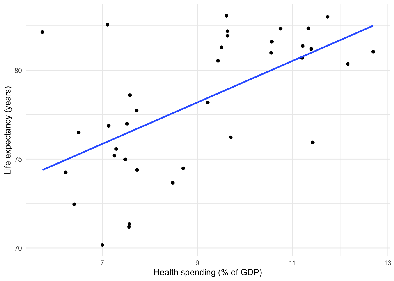
| Health spending (% of GDP) | 1.2 | 0.53, 1.9 | <0.001 |
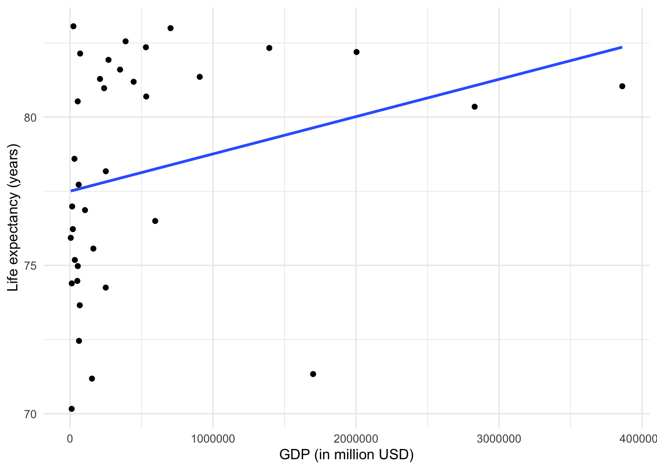
| GDP (in million USD) | 0.00 | 0.00, 0.00 | 0.9 |
| 1 CI = Confidence Interval | |||
- Plot each relationship in the regression model using
geom_smooth().
## `geom_smooth()` using formula = 'y ~ x'
europe_data |> ggplot(aes(x = gdp_md, y = years_to_live)) +
  geom_point() +
  geom_smooth(method = "lm", se = FALSE) +
  labs(
    x = "GDP (in million USD)",
    y = "Life expectancy (years)"
  ) +
  theme_minimal()
## `geom_smooth()` using formula = 'y ~ x'
And that’s science! All that would be left for you to do is write up your results and submit them to a journal.