Chapter 7 Lab 5 - 04/04/2023
In this lecture we will learn:
- how to reshape data from a wide to a long data format
- how to plot the kernel density estimate (KDE) together with an histogram
- how to compute the skewness and the kurtosis indexes
- how to plot the Normal probability plot
- how to test the normality using the Jarqe-Berta test
- how to fit a Normal distribution
For this lab the tidyverse package is required and loaded:
library(tidyverse)Also the moments package is required for computing the skewness/kurtosis and implementing the Jarque-Bera test:
library(moments)Finally, forcats is used for reordering labels in ggplot:
library(forcats)7.1 Data import
We have some financial data (i.e. prices) available in the Excel file named AdjclosepricesLab4Exercises.xlsx. It is possible to use the user-friendly feature provided by RStudio, as described in the previous lab (see section 6.1).
library(readxl)
prices <- read_excel("./files/AdjclosepricesLab4Exercises.xlsx")
glimpse(prices)
## Rows: 5,773
## Columns: 3
## $ ref.date <dttm> 2022-03-29, 2022-03-30, 2022-03-31, 2022-04-01, 2022-0…
## $ ticker <chr> "APA", "APA", "APA", "APA", "APA", "APA", "APA", "APA",…
## $ price.adjusted <dbl> 40.23189, 40.46763, 40.59532, 41.46950, 42.21598, 40.94…We realize that prices contains only three columns. We can check how many assets we have by computing the frequency distribution of ticker:
prices %>% count(ticker) %>% print(n=Inf)## # A tibble: 23 × 2
## ticker n
## <chr> <int>
## 1 APA 251
## 2 BKR 251
## 3 COP 251
## 4 CTRA 251
## 5 CVX 251
## 6 DVN 251
## 7 EOG 251
## 8 EQT 251
## 9 FANG 251
## 10 HAL 251
## 11 HES 251
## 12 KMI 251
## 13 MPC 251
## 14 MRO 251
## 15 OKE 251
## 16 OXY 251
## 17 PSX 251
## 18 PXD 251
## 19 SLB 251
## 20 TRGP 251
## 21 VLO 251
## 22 WMB 251
## 23 XOM 251We have 23 assets each repeated for 251 days (one financial year). Note that the option print(n=Inf) is used only for printing all the rows in the Console without any row being left out for the sake of space. The considered dates can be retrieved as follows:
prices %>% summarise(max(ref.date), min(ref.date))## # A tibble: 1 × 2
## `max(ref.date)` `min(ref.date)`
## <dttm> <dttm>
## 1 2023-03-28 00:00:00 2022-03-29 00:00:00The data are structured in the so-called long format (see also Section 6.3). In the long format, each row corresponds to a specific time point per asset. So each asset will have data in multiple rows.
7.2 From long to wide format
By using the following code it is possible to move from the long to the wide format:
prices_wide = prices %>%
  pivot_wider(names_from = ticker,
              values_from = price.adjusted)
glimpse(prices_wide)
## Rows: 251
## Columns: 24
## $ ref.date <dttm> 2022-03-29, 2022-03-30, 2022-03-31, 2022-04-01, 2022-04-04, …
## $ APA <dbl> 40.23189, 40.46763, 40.59532, 41.46950, 42.21598, 40.94892, 4…
## $ BKR <dbl> 35.75806, 36.42115, 35.50454, 35.51428, 35.52404, 34.63667, 3…
## $ CVX <dbl> 158.8675, 159.9890, 157.4269, 158.7708, 158.9158, 157.9393, 1…
## $ COP <dbl> 95.33895, 96.01321, 94.96857, 95.51939, 95.49091, 93.11669, 9…
## $ CTRA <dbl> 25.02817, 24.75414, 24.63539, 24.75414, 24.27915, 24.09647, 2…
## $ DVN <dbl> 55.93297, 55.97919, 54.65736, 55.78507, 56.24725, 54.04728, 5…
## $ FANG <dbl> 127.9130, 128.3003, 126.3917, 127.6456, 128.7059, 124.9164, 1…
## $ EOG <dbl> 112.1561, 112.5838, 110.8545, 111.8772, 112.3420, 109.5528, 1…
## $ EQT <dbl> 33.50015, 33.65776, 33.89415, 35.48987, 35.81492, 35.68687, 3…
## $ XOM <dbl> 79.49367, 80.85442, 79.70598, 80.21748, 80.25608, 79.84110, 8…
## $ HAL <dbl> 37.30344, 37.96377, 37.32315, 38.02290, 38.21016, 36.98806, 3…
## $ HES <dbl> 106.3883, 107.2478, 105.7461, 107.6726, 108.3839, 106.3290, 1…
## $ KMI <dbl> 17.77208, 17.96025, 17.79090, 18.08255, 18.15782, 17.80031, 1…
## $ MRO <dbl> 24.68381, 25.17749, 24.79242, 25.42433, 25.35521, 24.48634, 2…
## $ MPC <dbl> 81.15273, 83.30990, 83.45631, 82.78281, 83.03660, 82.68520, 8…
## $ OXY <dbl> 56.29007, 56.97400, 56.24051, 57.59845, 57.28127, 55.22949, 5…
## $ OKE <dbl> 67.13908, 67.58203, 66.56420, 67.31815, 67.07311, 65.81968, 6…
## $ PSX <dbl> 80.19965, 84.01411, 83.00525, 82.59209, 83.27428, 82.54407, 8…
## $ PXD <dbl> 226.4631, 230.5025, 223.4425, 226.2307, 225.8733, 218.4827, 2…
## $ SLB <dbl> 41.93759, 41.52441, 40.63902, 41.01285, 40.87513, 39.80283, 4…
## $ TRGP <dbl> 73.37575, 74.75817, 73.99343, 75.82684, 75.48370, 74.22873, 7…
## $ VLO <dbl> 93.71871, 97.42171, 98.42986, 98.16811, 97.65436, 98.35230, 1…
## $ WMB <dbl> 31.74527, 31.94463, 31.71679, 32.11550, 32.02057, 31.30858, 3…We see that the new data frame prices_wide contains more columns (one for each asset plus one for the date) and less rows (given by the number of financial days). We use this data frame to compute log-returns as described in Section 6.4:
# Compute log-prices
logprices = prices_wide %>% mutate(across(APA:WMB, log))

# Compute log-returns
logret = logprices %>% mutate(across(APA:WMB, ~ . - lag(.)))
glimpse(logret)
## Rows: 251
## Columns: 24
## $ ref.date <dttm> 2022-03-29, 2022-03-30, 2022-03-31, 2022-04-01, 2022-04-04, …
## $ APA <dbl> NA, 0.005842331, 0.003150492, 0.021305331, 0.017840748, -0.03…
## $ BKR <dbl> NA, 0.0183739495, -0.0254892967, 0.0002744625, 0.0002746124, …
## $ CVX <dbl> NA, 0.0070345730, -0.0161436617, 0.0085003460, 0.0009128745, …
## $ COP <dbl> NA, 0.0070473808, -0.0109398647, 0.0057833422, -0.0002982876,…
## $ CTRA <dbl> NA, -0.011009322, -0.004808639, 0.004808639, -0.019374666, -0…
## $ DVN <dbl> NA, 0.0008261301, -0.0238962963, 0.0204224991, 0.0082508976, …
## $ FANG <dbl> NA, 0.003023070, -0.014987791, 0.009872324, 0.008272483, -0.0…
## $ EOG <dbl> NA, 0.003806076, -0.015479522, 0.009183565, 0.004146546, -0.0…
## $ EQT <dbl> NA, 0.004693663, 0.006999002, 0.046004809, 0.009117262, -0.00…
## $ XOM <dbl> NA, 0.0169729325, -0.0143057139, 0.0063969068, 0.0004810387, …
## $ HAL <dbl> NA, 0.017546684, -0.017018346, 0.018574804, 0.004912629, -0.0…
## $ HES <dbl> NA, 0.0080462698, -0.0141004024, 0.0180535374, 0.0065843776, …
## $ KMI <dbl> NA, 0.010531960, -0.009473781, 0.016260461, 0.004153716, -0.0…
## $ MRO <dbl> NA, 0.019802658, -0.015412260, 0.025168509, -0.002722240, -0.…
## $ MPC <dbl> NA, 0.026234492, 0.001755944, -0.008102926, 0.003061068, -0.0…
## $ OXY <dbl> NA, 0.012076863, -0.012957708, 0.023858360, -0.005521981, -0.…
## $ OKE <dbl> NA, 0.006575786, -0.015175224, 0.011263022, -0.003646685, -0.…
## $ PSX <dbl> NA, 0.046465608, -0.012080962, -0.004989885, 0.008225824, -0.…
## $ PXD <dbl> NA, 0.017679481, -0.031107320, 0.012401198, -0.001581282, -0.…
## $ SLB <dbl> NA, -0.009901162, -0.021552588, 0.009156621, -0.003363672, -0…
## $ TRGP <dbl> NA, 0.018664950, -0.010282198, 0.024476040, -0.004535673, -0.…
## $ VLO <dbl> NA, 0.038751180, 0.010295112, -0.002662705, -0.005247173, 0.0…
## $ WMB <dbl> NA, 0.0062602915, -0.0071578042, 0.0124927732, -0.0029604578,…# Remove the NAs for the first day
logret = na.omit(logret)
glimpse(logret)## Rows: 250
## Columns: 24
## $ ref.date <dttm> 2022-03-30, 2022-03-31, 2022-04-01, 2022-04-04, 2022-04-05, …
## $ APA <dbl> 0.005842331, 0.003150492, 0.021305331, 0.017840748, -0.030473…
## $ BKR <dbl> 0.0183739495, -0.0254892967, 0.0002744625, 0.0002746124, -0.0…
## $ CVX <dbl> 0.0070345730, -0.0161436617, 0.0085003460, 0.0009128745, -0.0…
## $ COP <dbl> 0.0070473808, -0.0109398647, 0.0057833422, -0.0002982876, -0.…
## $ CTRA <dbl> -0.011009322, -0.004808639, 0.004808639, -0.019374666, -0.007…
## $ DVN <dbl> 0.0008261301, -0.0238962963, 0.0204224991, 0.0082508976, -0.0…
## $ FANG <dbl> 0.003023070, -0.014987791, 0.009872324, 0.008272483, -0.02988…
## $ EOG <dbl> 0.003806076, -0.015479522, 0.009183565, 0.004146546, -0.02514…
## $ EQT <dbl> 0.004693663, 0.006999002, 0.046004809, 0.009117262, -0.003581…
## $ XOM <dbl> 0.0169729325, -0.0143057139, 0.0063969068, 0.0004810387, -0.0…
## $ HAL <dbl> 0.017546684, -0.017018346, 0.018574804, 0.004912629, -0.03250…
## $ HES <dbl> 0.0080462698, -0.0141004024, 0.0180535374, 0.0065843776, -0.0…
## $ KMI <dbl> 0.010531960, -0.009473781, 0.016260461, 0.004153716, -0.01988…
## $ MRO <dbl> 0.0198026583, -0.0154122603, 0.0251685093, -0.0027222399, -0.…
## $ MPC <dbl> 0.026234492, 0.001755944, -0.008102926, 0.003061068, -0.00424…
## $ OXY <dbl> 0.012076863, -0.012957708, 0.023858360, -0.005521981, -0.0364…
## $ OKE <dbl> 0.006575786, -0.015175224, 0.011263022, -0.003646685, -0.0188…
## $ PSX <dbl> 0.046465608, -0.012080962, -0.004989885, 0.008225824, -0.0088…
## $ PXD <dbl> 0.017679481, -0.031107320, 0.012401198, -0.001581282, -0.0332…
## $ SLB <dbl> -0.009901162, -0.021552588, 0.009156621, -0.003363672, -0.026…
## $ TRGP <dbl> 0.018664950, -0.010282198, 0.024476040, -0.004535673, -0.0167…
## $ VLO <dbl> 0.038751180, 0.010295112, -0.002662705, -0.005247173, 0.00712…
## $ WMB <dbl> 0.0062602915, -0.0071578042, 0.0124927732, -0.0029604578, -0.…# Reshape from wide to long format
logret_long = logret %>% pivot_longer(APA:WMB)
glimpse(logret_long)## Rows: 5,750
## Columns: 3
## $ ref.date <dttm> 2022-03-30, 2022-03-30, 2022-03-30, 2022-03-30, 2022-03-30, …
## $ name <chr> "APA", "BKR", "CVX", "COP", "CTRA", "DVN", "FANG", "EOG", "EQ…
## $ value <dbl> 0.0058423314, 0.0183739495, 0.0070345730, 0.0070473808, -0.01…We finally plot the log-returns time series:
logret_long %>%
  ggplot() +
  geom_line(aes(ref.date, value, col=name)) +
  ylab("Log-returns")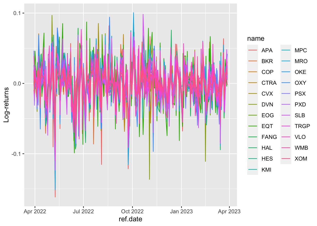
7.3 Histogram and Kernel Density Estimate
The log-returns of the 23 assets can be represented graphically by using histograms (using facet_wrap to create sub-plots, one for each asset):
logret_long %>%
  ggplot() +
  geom_histogram(aes(value, fill=name)) +
  facet_wrap(~name)
## `stat_bin()` using `bins = 30`. Pick better value with `binwidth`.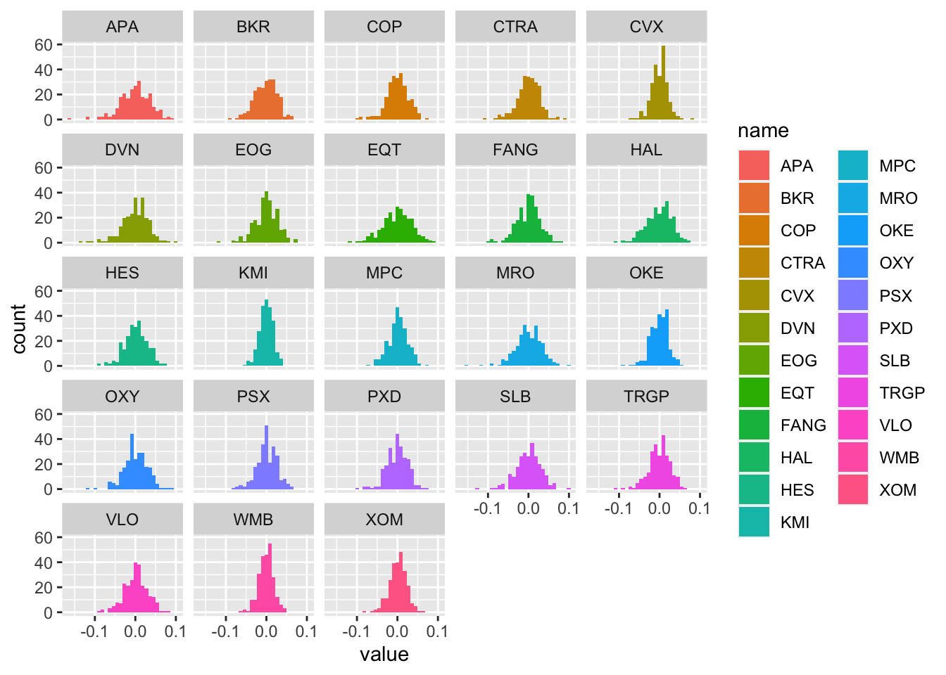 The plot represents the values of the log-returns on the x-axis (with classes of values set automatically by R) and the corresponding frequencies (i.e. number of days) on the y-axis (denoted as
 count). From the histograms we observe peaked/wide distributions and distribution with extreme values.
The plot of the Kernel Density Estimate (KDE) can be obtained by using the geom_density geometry (the bandwith parameter is set automatically):
logret_long %>%
  ggplot() +
  geom_density(aes(value, fill=name)) +
  facet_wrap(~name)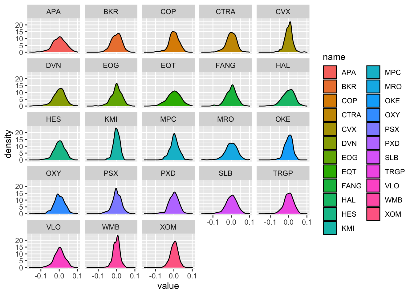
It is also possible to plot together the histogram and the KDE line by combining together 2 geometries. In this case the histogram will have to be plotted by using densities in the y-axis instead of counts (this can be obtained by using ..density.. as second argument inside aes()):
logret_long %>%
  ggplot() +
  geom_histogram(aes(value, ..density..), col="black") +
  geom_density(aes(value, fill=name), alpha=0.2) + #alpha is used for transparency
  facet_wrap(~name) +
  theme(legend.position="none") #remove legend on the right
## `stat_bin()` using `bins = 30`. Pick better value with `binwidth`.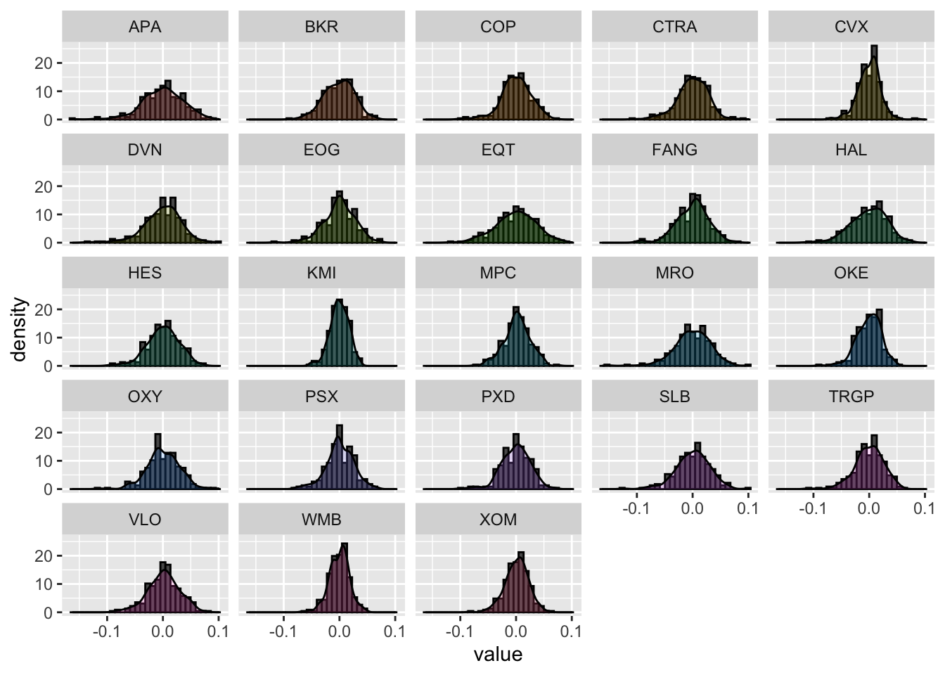 Note that in the density histogram the area of each single bar is represented by the absolute frequency of that class of values.
7.4 Skewness and Kurtosis with long shaped data
We start by computing skewness and kurtosis using the long format data through the function skewness and kurtosis from the moments package. We will basically combine the
group_by function with the summarise verb in order to compute summary statistics conditionally on the asset names:
SK = logret_long %>%
  group_by(name) %>%
  summarise(sk = skewness(value),
            kur = kurtosis(value))
SK
## # A tibble: 23 × 3
## name sk kur
## <chr> <dbl> <dbl>
## 1 APA -0.547 4.35
## 2 BKR -0.228 2.88
## 3 COP -0.505 4.11
## 4 CTRA -0.415 4.08
## 5 CVX -0.142 4.65
## 6 DVN -0.632 4.57
## 7 EOG -0.425 3.88
## 8 EQT -0.247 3.06
## 9 FANG -0.449 3.86
## 10 HAL -0.423 3.29
## # … with 13 more rowsFor each asset we know the skewness and the kurtosis values. We start by plotting the skewness values by using the geom_col geometry (this is an alternative to geom_bar when the y-axis should not by given by count automatically but by another variable, here sk for example):
SK %>%
  ggplot() +
  geom_col(aes(name, sk))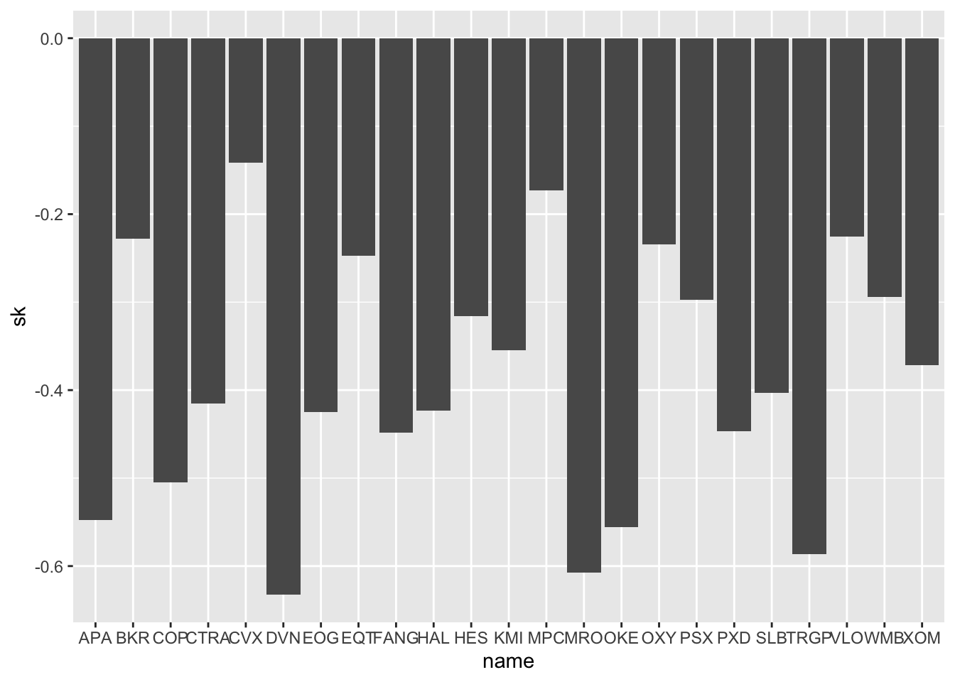
We note that all the skewnesses are negative (left asymmetry). It would be nice to have bars ordered b the skewness value. In this regard we can use the function fct_reorder (from the forcats package) for reordering the categories name according to sk values:
SK %>%
  ggplot() +
  geom_col(aes(fct_reorder(name,sk), sk))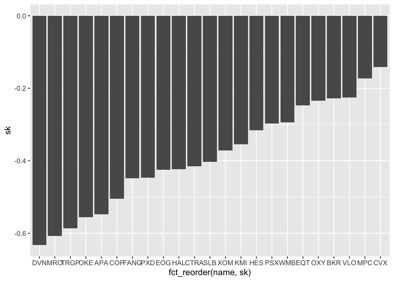
The asset with the highest negative asymmetry is DVN. The with the value of the skewness closer to zero is CVX.
We now plot together with a scatterplot skewness and kurtosis:
SK %>%
ggplot() +
geom_point(aes(sk, kur)) +
geom_text(aes(sk, kur, label=name))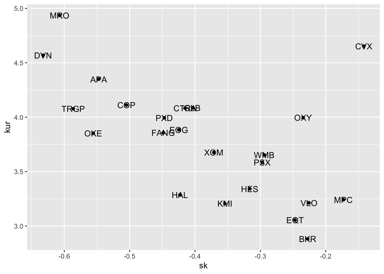 where the geometry
 geom_text is used for including labels - given by name in the scatterplot. Note that the aes settings can be specified separately for each layer or globally in the ggplot() function. See here below for a different specification (global now) of the previous plot:
SK %>%
  ggplot(aes(sk, kur)) +
  geom_point() +
  geom_text(aes(label=name))
7.5 Skewness and Kurtosis with wide shaped data
To compute the two indexes for all the assets, which are represented as separate columns in the wide data format, we combine summarise together with across, as follows:
logret %>%
  summarise(across(APA:WMB, skewness))
## # A tibble: 1 × 23
## APA BKR CVX COP CTRA DVN FANG EOG EQT XOM HAL
## <dbl> <dbl> <dbl> <dbl> <dbl> <dbl> <dbl> <dbl> <dbl> <dbl> <dbl>
## 1 -0.547 -0.228 -0.142 -0.505 -0.415 -0.632 -0.449 -0.425 -0.247 -0.371 -0.423
## # … with 12 more variables: HES <dbl>, KMI <dbl>, MRO <dbl>, MPC <dbl>,
## # OXY <dbl>, OKE <dbl>, PSX <dbl>, PXD <dbl>, SLB <dbl>, TRGP <dbl>,
## # VLO <dbl>, WMB <dbl>logret %>%
summarise(across(APA:WMB, kurtosis))## # A tibble: 1 × 23
## APA BKR CVX COP CTRA DVN FANG EOG EQT XOM HAL HES KMI
## <dbl> <dbl> <dbl> <dbl> <dbl> <dbl> <dbl> <dbl> <dbl> <dbl> <dbl> <dbl> <dbl>
## 1 4.35 2.88 4.65 4.11 4.08 4.57 3.86 3.88 3.06 3.68 3.29 3.34 3.21
## # … with 10 more variables: MRO <dbl>, MPC <dbl>, OXY <dbl>, OKE <dbl>,
## # PSX <dbl>, PXD <dbl>, SLB <dbl>, TRGP <dbl>, VLO <dbl>, WMB <dbl>7.6 Normal probability plot
Here after we consider only BKR as asset (located in the bottom right part of the scatterplot). We are going to study further its distribution. In this case it is more convenient to use the wide data and to extract the required information with logret$BKR.
The normal probability plot is a graphical tool to study the normality of a distribution. It is based on the comparison between the sample (empirical) quantiles (usually represented on the x-axis) and the quantiles of a standard Normal distribution (usually represented on the y-axis). If the normality assumption is met, the sample quantiles are approximately equal to the Normal quantiles and the points in the plot are linearly distributed. If the normality assumpation is not compatible with the data, 4 possible cases can occur, as displayed in Figure 7.1.
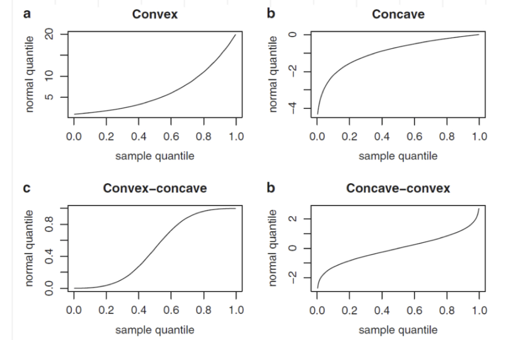
Figure 7.1: Patterns of the normal probability plots in case of non normality: a = left skewness, b = right skewness, c = heavier tails, d = lighter tails
In R the function for producing the normal probability plot is qqnorm:
qqnorm(logret$BKR)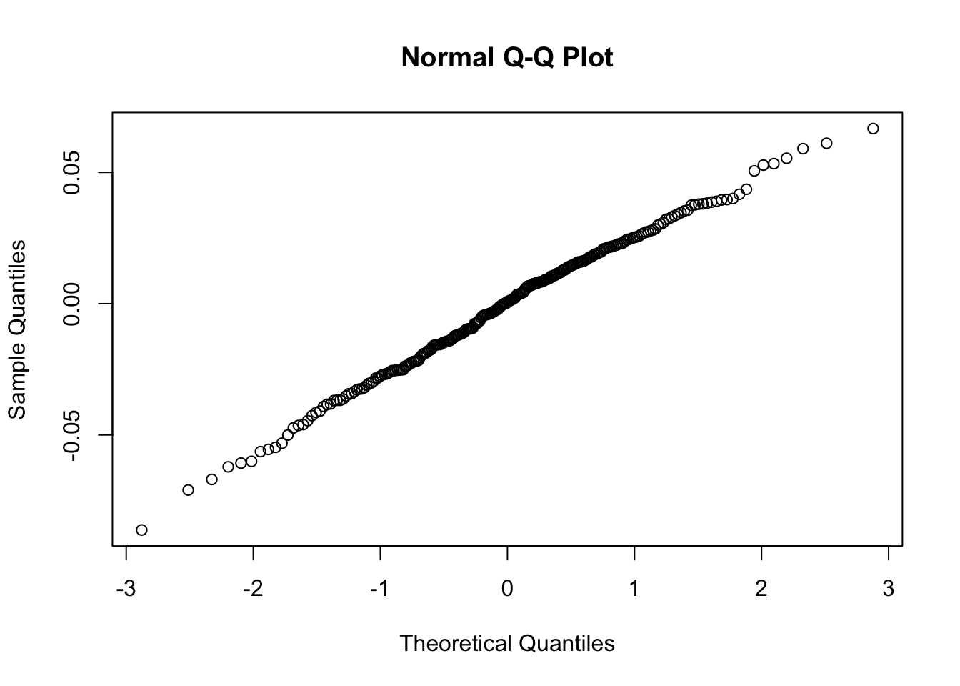 Note that this plot, differently from what reported in Figure 7.1, reports on the x-axis the theoretical Normal quantiles. So pay attention to what you have on the axes, otherwise your comments coulb be completely wrong, as shown in Figure 7.2 😄.
Figure 7.2: Check the axes!
In order to exchange the axes, it is possible to use the datax option of the qqnorm function, as follows. Moreover, it is also useful to include a reference straight line by using qqline.
qqnorm(logret$BKR, datax=T)
qqline(logret$BKR, datax=T)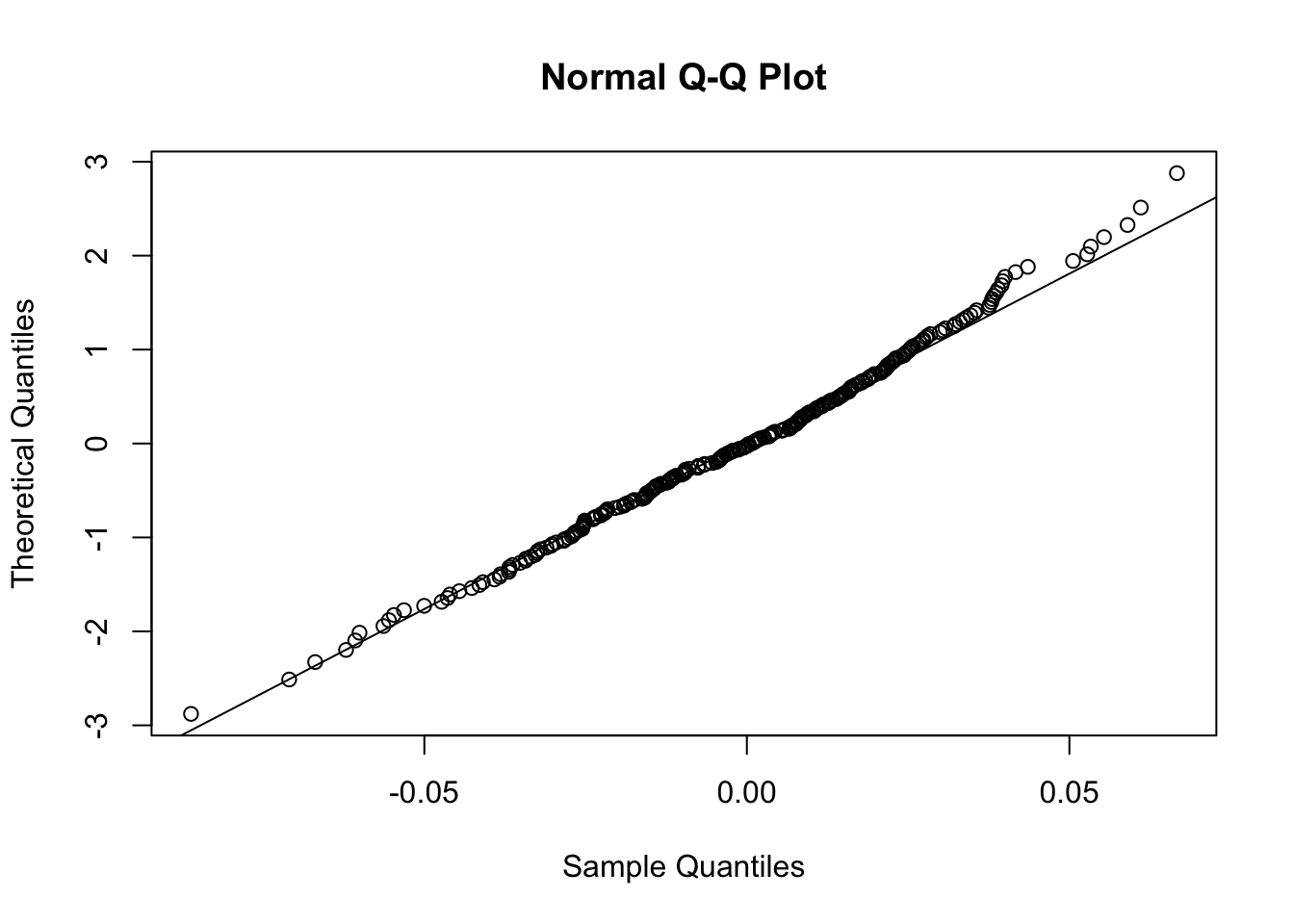
Figure 7.3: Normal probability plot for the data in the y vector
The reference straight line goes through the pair of first quartiles and the pair of third quartiles. Moreover, the sample quantiles are given by the ordered data \(y_{(i)}\) (for \(i=1,\ldots, n\)), while the theoretical quantiles are given by the \(\Phi^{-1}\left(\frac{i-0.5}{n}\right)\) (for \(i=1,\ldots, n\)), where \(\Phi^{-1}\) is the inverse of the cumulative distribution function of the Normal distribution (i.e. the quantile function the Normal distribution). The data are align along the straight line; this suggests that the data could have been generated by a normal distribution.
7.7 Jarque-Bera Normality test
The Jarque-bera test of normality uses the sample skewness \(\hat{Sk}\) and kurtosis \(\hat{Kur}\) which are compared with the corresponding expected value (0 and 3) in case of Normal distribution. The test statistic is given by \[ JB = n\left (\frac{\hat{Sk}^2}{6}+\frac{(\hat{Kur}-3)^2}{24}\right) \] which, under the null hypothesis, is approximately distributed like a Chi-square distribution with 2 degrees of freedom (\(\chi^2_2\)). Under the null hypothesis (normality), we expect a value of the test statistic close to 0.
This test is implemented in R using the jarque.test function which is part of the moments package.
jarque.test(logret$BKR)##
## Jarque-Bera Normality Test
##
## data: logret$BKR
## JB = 2.305, p-value = 0.3159
## alternative hypothesis: greaterGiven the extremely large value of the p-value, we do not reject, as expected given the previous plots, the normality hypothesis which is supported by the data.
7.8 Fit a distribution to the data
In this Section we learn to fit a distribution, whose probability density function (PDF) is known (e.g. Normal distribution or t distribution), to the data. The parameters of the theoretical model are estimated by using the maximum likelihood (ML) approach. The function in R for this analysis is called fitdistr and it is contained in the MASS library. The latter is already available in the standard release of R and it is not necessary to install it; you just have to load it. The inputs of fitdistr are: the data and the theoretical chosen model (see ?fitdistr for the available options). Let’s consider first the case of the Normal distribution:
library(MASS) #load the library##
## Attaching package: 'MASS'## The following object is masked from 'package:dplyr':
##
## selectfitN = fitdistr(logret$BKR, densfun="normal")
fitN## mean sd
## -0.001038740 0.026890575
## ( 0.001700709) ( 0.001202583)The output of fitN provides the ML estimates of the parameters of the Normal distribution (in this case mean \(\mu\) and sd \(\sigma\)) with the corresponding standard errors provided in parentheses (i.e. the standard deviation of the ML estimates) which represent a measure of accuracy of the estimates (the lower the better). In case of Normal model, the ML of the mean \(\mu\) is given by the sample mean \(\bar x=\frac{\sum_{i=1}^n x_i}{n}\), while the ML of the variance is given by the biased sample variance \(s^2 =\frac{\sum_{i=1}^n (x_i-\bar x)^2}{n}\).
Note from the top-right panel that the object fitN is a list (this is a new kind of object for us1) containing 5 elements that can be displayed using
names(fitN)## [1] "estimate" "sd" "vcov" "n" "loglik"To extract one element from a list we use the dollar; for example to extract from fitN the object containing the parameter estimates:
fitN$estimate #vector of estimates## mean sd
## -0.00103874 0.02689058fitN$estimate[1] #first estimate## mean
## -0.00103874fitN$estimate[2] #second estimate## sd
## 0.02689058Another distribution can be fitted to the data, such as for example the (so called standardized) t distribution \(t_\nu^{std}(\mu,\sigma^2)\). Note that in this case three parameters are estimated using the ML approach: mean \(\mu\), sd \(\sigma\) and degrees of freedom \(\nu\) (df):
fitt = fitdistr(logret$BKR,"t")## Warning in log(s): NaNs produced
## Warning in log(s): NaNs produced
## Warning in log(s): NaNs produced
## Warning in log(s): NaNs produced
## Warning in log(s): NaNs produced
## Warning in log(s): NaNs produced
## Warning in log(s): NaNs produced
## Warning in log(s): NaNs produced
## Warning in log(s): NaNs produced
## Warning in log(s): NaNs produced
## Warning in log(s): NaNs produced
## Warning in log(s): NaNs produced
## Warning in log(s): NaNs produced
## Warning in log(s): NaNs produced
## Warning in log(s): NaNs produced
## Warning in log(s): NaNs produced
## Warning in log(s): NaNs produced
## Warning in log(s): NaNs produced
## Warning in log(s): NaNs produced
## Warning in log(s): NaNs produced
## Warning in log(s): NaNs producedfitt## m s df
## -0.0009212099 0.0263955139 48.9524562592
## ( 0.0017079846) ( 0.0013379453) (60.0820757115)7.8.1 AIC and BIC
Which is the best model between the Normal and the t distribution? To compare them we can use the log likelihood value of the two fitted model (which is provided as loglik in the output of fitdistr): the higher the better.
fitN$loglik## [1] 549.2602fitt$loglik ## [1] 549.0458In this case the t distribution has a higher log likelihood value. A similar conclusion is obtained by using the deviance which is a misfit index that should be minimized (the smaller the deviance the better the fit): the deviance is given by \[\text{deviance} = -2*\text{loglikelihood}.\]
-2*fitN$loglik## [1] -1098.52-2*fitt$loglik ## [1] -1098.092Again the t distribution performs better in term of goodness of fit but it is also a more complex model (one extra parameter to estimate). Can we consider also model complexity? The Akaike Information Criterion (AIC) and the Bayes information criterion (BIC) indexes take into account model complexity by penalizing for the number of parameters to be estimated: \[ AIC = \text{deviance}+2p \]
\[ BIC = \text{deviance}+\log(n)p \] where \(p\) is the numbers of estimated parameters (2 for the Normal model and 3 for the t distribution) and \(n\) the sample size. The terms \(2p\) and \(\log(n)p\) are called complexity penalties.
Both AIC and BIC follow the criterion smaller is better, since small values of AIC and BIC tend to minimize both the deviance and model complexity. Note that usually \(\log(n)>2\), thus BIC penalizes model complexity more than AIC. For this reason, BIC tends to select simpler models.
#### AIC ####
#AIC for the normal model
-2*fitN$loglik + 2* length(fitN$estimate)
## [1] -1094.52#AIC for the t model
-2*fitt$loglik + 2* length(fitt$estimate)## [1] -1092.092#### BIC ####
#BIC for the normal model
-2*fitN$loglik + log(length(logret)) * length(fitN$estimate)## [1] -1092.164#BIC for the t model
-2*fitt$loglik + log(length(logret)) * length(fitt$estimate)## [1] -1088.557The two indexes can be computed also by using the R functions AIC and BIC:
AIC(fitN)## [1] -1094.52AIC(fitt)## [1] -1092.092BIC(fitN)## [1] -1087.478BIC(fitt)## [1] -1081.527If we compare the AIC and BIC values we prefer the t model, which outperforms the Normal model also when adjusting by model complexity.
7.8.2 Plot of the density function of the Normal distribution
Let’s compare graphically the KDE of logret with the Normal PDF fitted to the data given by the following formula (the parameters \(\mu\) and \(\sigma^2\) are substituted by the corresponding estimates \(\bar x\) and \(s^2\)):
\[
\hat f(x)=\frac{1}{\sqrt{2\pi s^2}}e^{-\frac{1}{s^2}(x-\bar x)^2}
\]
Usually to compute the PDF values we use the dnorm(x,mean,sd) function which returns the values of the Normal probability density function evaluated for a set of values x. This dnorm function can be used in a ggplot geometry named geom_function which requires the specification of the two arguments (mean and sd) included in a list:
logret %>%
  ggplot() +
  geom_density(aes(BKR)) +
  geom_function(fun = dnorm,
                args = list(mean = fitN$estimate[1], sd=fitN$estimate[2]),
                colour = "red")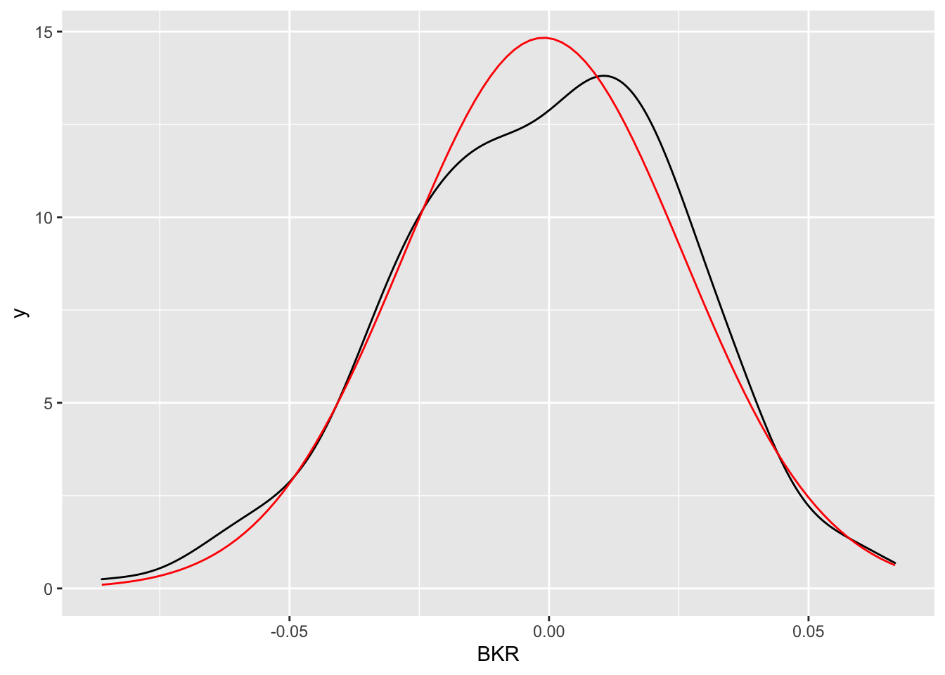
The two functions (empirical and estimated density) are quite similar.
7.9 Exercises Lab 5
7.9.1 Exercise 1
Import in R the data available in the GDAXI.csv file. The data refer to the DAX index which is computed considering 30 major German companies trading on the Frankfurt Stock Exchange. Check how the data look like and their structure.
Using a scatterplot to display
OpenandCloseprices. Comment the plot.Plot the time series of
Adj.Closeprices (with dates on the x-axis, you need to uselubridateto set them correctly). Do you think the price time series is stationary in time?Create in the dataframe a new column containing the month for each observation. Compute the average
Volumeconditionally on the month. Find the month with the highest average volume.Using
Adj.Closecompute the DAX gross returns (note that in this case you are working with one column only) and plot the obtained time series. Do you think the return time series is stationary in time? Remember also to remove the missing value corresponding to the first day.Use the histogram to study the gross returns. Add to the histogram the KDE line.
Compute the skewness and the kurtosis for the gross returns. Comment the values.
Provide the normal probability plot. Comment the plot.
Fit the Normal and t distribution to the gross returns data. Provide the estimated parameters. Moreover, which is the best model by using the AIC?
Perform the Jarque-Bera test. Which is your conclusion? Explain why.
Lists are another kind of objects for data storage. Lists have elements, each of which can contain any type of
Robject, i.e. the elements of a list do not have to be of the same type.↩︎