Chapter 5 Lab 3 - 22/03/2023
In this lecture we will learn:
- how to import data from a csv file
- some functions from the tidyverse package to work with dates
- the remaining tidyverse verbs
- how to plot a time series with ggplot
For this lab the following packages are required and loaded (obviously this means that you have already installed them in the past):
library(tidyverse)
library(lubridate) #for date manipulation
##
## Attaching package: 'lubridate'## The following objects are masked from 'package:base':
##
## date, intersect, setdiff, union5.1 Data import
We have some financial data (i.e. prices) available in the csv file named Adjcloseprices27012023.csv. Note that a csv file can be open using a text editor (e.g. TextNote, TextEdit), see Figure 5.1.
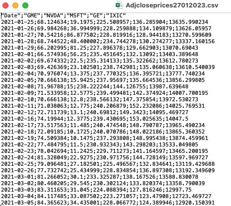
Figure 5.1: Preview using TextEdit of the csv file containing financial data
There are 3 things that characterize a csv file:
- the header: the first line containing the names of the variables;
- the field separator (delimiter): the character separating the information (usually the semicolon or the comma is used);
- the decimal separator: the character used for real number decimal points (it can be the full stop or the comma).
In the preview of the csv file reported in Figure 5.1
- the header is given by a set of text strings:
- “;” is the field separator;
- “.” is the decimal separator.
All this information are required when importing the data in R by using the read.csv function, whose main arguments are reported here below (see ?read.csv):
file: the name of the file which the data are to be read from; this can also including the specification of the folder path (use quotes to specify it);header: a logical value (TorF) indicating whether the file contains the names of the variables as its first line;sep: the field separator character (use quotes to specify it);dec: the character used in the file for decimal points (use quotes to specify it).
The following code is used to import the data available in the Adjcloseprices.csv file. The output is an object named prices:
prices <- read.csv("files/Adjcloseprices27012023.csv", sep=";")The argument header=T and dec="." are set to the default value (see ?read.csv) and they could be omitted.
Alternatively, it is possible to use the user-friendly feature provided by RStudio: read here for more information. The data import feature can be accessed from the environment (top-right) panel (see Figure 5.2). Then all the necessary information can be specified in the following Import Dataset window as shown in Figure 5.3.
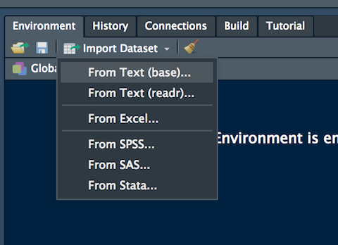
Figure 5.2: The Import Dataset feature of RStudio
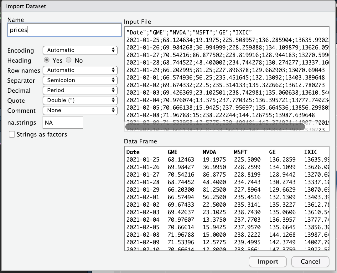
Figure 5.3: Specification of the csv file characteristics through the Import Dataset feature
After clicking on Import an object named prices will be created (essentially this RStudio feature makes use of the read.csv function).
The prices is an object of class data.frame:
class(prices)## [1] "data.frame"Data frames are matrix of data where you can find subjects (in this case each day) in the rows and variables in the column (in this case you have the following variables: dates, AAPL prices, etc.).
By using glimpse (from the tidyverse package) we get information about the type of variables included in the data frame:
glimpse(prices) ## Rows: 503
## Columns: 6
## $ Date <chr> "2021-01-25", "2021-01-26", "2021-01-27", "2021-01-28", "2021-01-…
## $ GME <dbl> 68.12463, 69.98427, 70.54216, 68.74452, 66.20300, 66.57494, 69.67…
## $ NVDA <dbl> 19.1975, 36.9950, 86.8775, 48.4000, 81.2500, 56.2500, 22.5000, 23…
## $ MSFT <dbl> 225.5090, 228.2599, 228.8199, 234.7443, 227.8964, 235.4516, 235.3…
## $ GE <dbl> 136.2859, 134.1099, 128.9442, 130.2743, 129.6629, 132.1309, 135.3…
## $ IXIC <dbl> 13635.99, 13626.06, 13270.60, 13337.16, 13070.69, 13403.39, 13612…In this case the variable Date is interpreted as text (chr stands for characters, a vector of strings) while the other variables (all the prices) are in the form of numerical variables.
It is possible to get a preview of the top or bottom part of the data frame by using head or tail:
head(prices) #preview of the first 6 lines (oldest data)## Date GME NVDA MSFT GE IXIC
## 1 2021-01-25 68.12463 19.1975 225.5090 136.2859 13635.99
## 2 2021-01-26 69.98427 36.9950 228.2599 134.1099 13626.06
## 3 2021-01-27 70.54216 86.8775 228.8199 128.9442 13270.60
## 4 2021-01-28 68.74452 48.4000 234.7443 130.2743 13337.16
## 5 2021-01-29 66.20300 81.2500 227.8964 129.6629 13070.69
## 6 2021-02-01 66.57494 56.2500 235.4516 132.1309 13403.39tail(prices) #preview of the last 6 lines (most recent data)## Date GME NVDA MSFT GE IXIC
## 498 2023-01-13 80.20 20.49 239.23 168.99 11079.16
## 499 2023-01-17 80.49 21.80 240.35 177.02 11095.11
## 500 2023-01-18 79.27 20.79 235.81 173.77 10957.01
## 501 2023-01-19 76.86 19.04 231.93 167.65 10852.27
## 502 2023-01-20 77.68 19.61 240.22 178.39 11140.43
## 503 2023-01-23 79.77 21.66 242.58 191.93 11364.41Note that the top of the data frame contains the oldest data while the bottom part of the data frame the most recent data.
Use the following alternative function if you want to get information about the dimensions of the data frame:
nrow(prices) #number of rows## [1] 503ncol(prices) #number of columns## [1] 6dim(prices) #no. of rows and columns## [1] 503 65.2 Working with dates
As mentioned in the previous section, it is necessary to transform the column Date so that the dates will be considered as actual dates and not as strings of text. To do this we will use the function ymd from the lubridate package. In particular, we will create a new column named DateOK:
prices$DateOK = ymd(prices$Date)
glimpse(prices)
## Rows: 503
## Columns: 7
## $ Date <chr> "2021-01-25", "2021-01-26", "2021-01-27", "2021-01-28", "2021-0…
## $ GME <dbl> 68.12463, 69.98427, 70.54216, 68.74452, 66.20300, 66.57494, 69.…
## $ NVDA <dbl> 19.1975, 36.9950, 86.8775, 48.4000, 81.2500, 56.2500, 22.5000, …
## $ MSFT <dbl> 225.5090, 228.2599, 228.8199, 234.7443, 227.8964, 235.4516, 235…
## $ GE <dbl> 136.2859, 134.1099, 128.9442, 130.2743, 129.6629, 132.1309, 135…
## $ IXIC <dbl> 13635.99, 13626.06, 13270.60, 13337.16, 13070.69, 13403.39, 136…
## $ DateOK <date> 2021-01-25, 2021-01-26, 2021-01-27, 2021-01-28, 2021-01-29, 20…Now DateOK is really a vector of dates! We don’t need the old column Date anymore. We can remove it using the tidyverse select verb as follows:
prices = prices %>% select(-Date)
glimpse(prices)
## Rows: 503
## Columns: 6
## $ GME <dbl> 68.12463, 69.98427, 70.54216, 68.74452, 66.20300, 66.57494, 69.…
## $ NVDA <dbl> 19.1975, 36.9950, 86.8775, 48.4000, 81.2500, 56.2500, 22.5000, …
## $ MSFT <dbl> 225.5090, 228.2599, 228.8199, 234.7443, 227.8964, 235.4516, 235…
## $ GE <dbl> 136.2859, 134.1099, 128.9442, 130.2743, 129.6629, 132.1309, 135…
## $ IXIC <dbl> 13635.99, 13626.06, 13270.60, 13337.16, 13070.69, 13403.39, 136…
## $ DateOK <date> 2021-01-25, 2021-01-26, 2021-01-27, 2021-01-28, 2021-01-29, 20…We now create a new column containing the month for each observation by means of the month function from lubridate:
prices$month = month(prices$DateOK)
glimpse(prices)
## Rows: 503
## Columns: 7
## $ GME <dbl> 68.12463, 69.98427, 70.54216, 68.74452, 66.20300, 66.57494, 69.…
## $ NVDA <dbl> 19.1975, 36.9950, 86.8775, 48.4000, 81.2500, 56.2500, 22.5000, …
## $ MSFT <dbl> 225.5090, 228.2599, 228.8199, 234.7443, 227.8964, 235.4516, 235…
## $ GE <dbl> 136.2859, 134.1099, 128.9442, 130.2743, 129.6629, 132.1309, 135…
## $ IXIC <dbl> 13635.99, 13626.06, 13270.60, 13337.16, 13070.69, 13403.39, 136…
## $ DateOK <date> 2021-01-25, 2021-01-26, 2021-01-27, 2021-01-28, 2021-01-29, 20…
## $ month <dbl> 1, 1, 1, 1, 1, 2, 2, 2, 2, 2, 2, 2, 2, 2, 2, 2, 2, 2, 2, 2, 2, …Similarly a new column named dow will be created containing the information about the day of the week (in particular 2 is Monday, 3 is Tuesday, … 6 is Friday - remember that we are speaking about a financial week):
prices$dow = wday(prices$DateOK)
glimpse(prices)
## Rows: 503
## Columns: 8
## $ GME <dbl> 68.12463, 69.98427, 70.54216, 68.74452, 66.20300, 66.57494, 69.…
## $ NVDA <dbl> 19.1975, 36.9950, 86.8775, 48.4000, 81.2500, 56.2500, 22.5000, …
## $ MSFT <dbl> 225.5090, 228.2599, 228.8199, 234.7443, 227.8964, 235.4516, 235…
## $ GE <dbl> 136.2859, 134.1099, 128.9442, 130.2743, 129.6629, 132.1309, 135…
## $ IXIC <dbl> 13635.99, 13626.06, 13270.60, 13337.16, 13070.69, 13403.39, 136…
## $ DateOK <date> 2021-01-25, 2021-01-26, 2021-01-27, 2021-01-28, 2021-01-29, 20…
## $ month <dbl> 1, 1, 1, 1, 1, 2, 2, 2, 2, 2, 2, 2, 2, 2, 2, 2, 2, 2, 2, 2, 2, …
## $ dow <dbl> 2, 3, 4, 5, 6, 2, 3, 4, 5, 6, 2, 3, 4, 5, 6, 3, 4, 5, 6, 2, 3, …5.3 summarise tidyverse verb
This verb can be used to compute summary statistics. For example the following code compute, separately for each variable, the following summary statistics:
- average of the GME prices
- median of the MSFT prices
- variance of the NVDA prices
- coefficient of variation of the GME prices (given by the ration between the standard deviation and the mean)
- the min and max of the DateOK vector (this is giving us information about the time window)
Note that it is possible to specify a personalized label for each summary statistics:
prices %>%
  summarise(avgGME = mean(GME),
            medMSFT = median(MSFT),
            var(NVDA),
            CVGME = sd(GME)/mean(GME),
            min(DateOK), max(DateOK))
## avgGME medMSFT var(NVDA) CVGME min(DateOK) max(DateOK)
## 1 71.19148 266.3425 146.1382 0.153238 2021-01-25 2023-01-23It is also interesting to compute summary statistics conditionally on the categories
of a qualitative/discrete variable. This can be done by combining the
group_by function with the summarise verb. Let’s compute for example the
mean price of GME conditionally on the month:
prices %>%
  group_by(month) %>%
  summarise(meanGME = mean(GME))
## # A tibble: 12 × 2
## month meanGME
## <dbl> <dbl>
## 1 1 75.0
## 2 2 74.5
## 3 3 76.9
## 4 4 76.0
## 5 5 70.4
## 6 6 69.3
## 7 7 66.1
## 8 8 69.8
## 9 9 66.5
## 10 10 67.8
## 11 11 73.3
## 12 12 68.9In this case the output is another data frame with 12 rows (the months) and the corresponding mean price of GME. Note that the data are ordered by month. It is also possible to arrange the rows by using the values of meanGME using the arrange tidyverse verb, as follows:
prices %>%
  group_by(month) %>%
  summarise(meanGME = mean(GME)) %>%
  arrange(meanGME) #ascending order
## # A tibble: 12 × 2
## month meanGME
## <dbl> <dbl>
## 1 7 66.1
## 2 9 66.5
## 3 10 67.8
## 4 12 68.9
## 5 6 69.3
## 6 8 69.8
## 7 5 70.4
## 8 11 73.3
## 9 2 74.5
## 10 1 75.0
## 11 4 76.0
## 12 3 76.9July (7) is the month with the lowest average price, march (3) is the month with the highes average price.
If you prefer a descending order use the following code (with the -):
prices %>%
  group_by(month) %>%
  summarise(meanGME = mean(GME)) %>%
  arrange(- meanGME)
## # A tibble: 12 × 2
## month meanGME
## <dbl> <dbl>
## 1 3 76.9
## 2 4 76.0
## 3 1 75.0
## 4 2 74.5
## 5 11 73.3
## 6 5 70.4
## 7 8 69.8
## 8 6 69.3
## 9 12 68.9
## 10 10 67.8
## 11 9 66.5
## 12 7 66.15.4 mutate tidyverse verb
The verb mutate can be used to create new column in the data frame. For example, let’s create a new variable transforming the GME prices (in dollar) into prices in euro (the exchange rate is 0.93).
prices = prices %>%
  mutate(GMEeuro = GME * 0.93)
glimpse(prices)
## Rows: 503
## Columns: 9
## $ GME <dbl> 68.12463, 69.98427, 70.54216, 68.74452, 66.20300, 66.57494, 69…
## $ NVDA <dbl> 19.1975, 36.9950, 86.8775, 48.4000, 81.2500, 56.2500, 22.5000,…
## $ MSFT <dbl> 225.5090, 228.2599, 228.8199, 234.7443, 227.8964, 235.4516, 23…
## $ GE <dbl> 136.2859, 134.1099, 128.9442, 130.2743, 129.6629, 132.1309, 13…
## $ IXIC <dbl> 13635.99, 13626.06, 13270.60, 13337.16, 13070.69, 13403.39, 13…
## $ DateOK <date> 2021-01-25, 2021-01-26, 2021-01-27, 2021-01-28, 2021-01-29, 2…
## $ month <dbl> 1, 1, 1, 1, 1, 2, 2, 2, 2, 2, 2, 2, 2, 2, 2, 2, 2, 2, 2, 2, 2,…
## $ dow <dbl> 2, 3, 4, 5, 6, 2, 3, 4, 5, 6, 2, 3, 4, 5, 6, 3, 4, 5, 6, 2, 3,…
## $ GMEeuro <dbl> 63.35591, 65.08537, 65.60421, 63.93241, 61.56879, 61.91469, 64…Note the new variable in the data frame named GMEeuro. The creation is permanent because we overwrite the old prices data frame (with prices = price %>% ...).
The function count can be used to get the frequency distribution of a qualitative/discrete variable, as for example dow:
prices %>%
  count(dow)
## dow n
## 1 2 92
## 2 3 104
## 3 4 104
## 4 5 102
## 5 6 101We obtain a small table with two columns: the first one refers to the day of the week, the second one (automatically named n) contains the corresponding absolute frequency. For example, 92 days (out of the 503) are Monday.
If you want to get percentages instead of absolute frequencies you can create a new variable using mutate:
prices %>%
  count(dow) %>%
  mutate(perc = n/sum(n) * 100)
## dow n perc
## 1 2 92 18.29026
## 2 3 104 20.67594
## 3 4 104 20.67594
## 4 5 102 20.27833
## 5 6 101 20.07952The sum of the percentages is 100.
5.5 The ggplot2 library
The ggplot2 is part of the tidyverse collection of packages. The grammar of graphics plot (ggplot) is an alternative to standard R functions for plotting; see here for the ggplot2 website. In Figure ?? we have some examples of plot (simple scatterplot, scatterplot with legend and boxplots) produced using standard R code and the ggplot2 library.
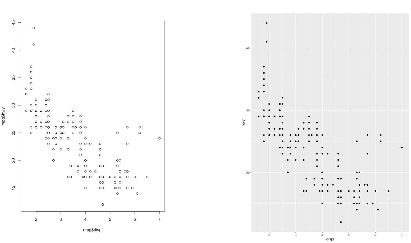
Figure 5.4: Comparison between standard and ggplot2 plots
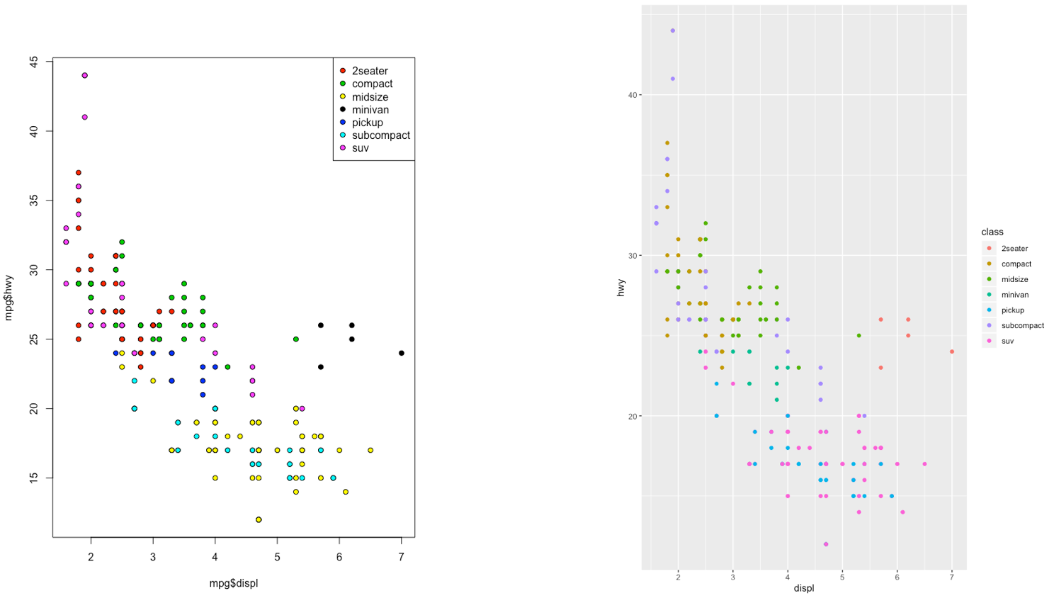
Figure 5.5: Comparison between standard and ggplot2 plots
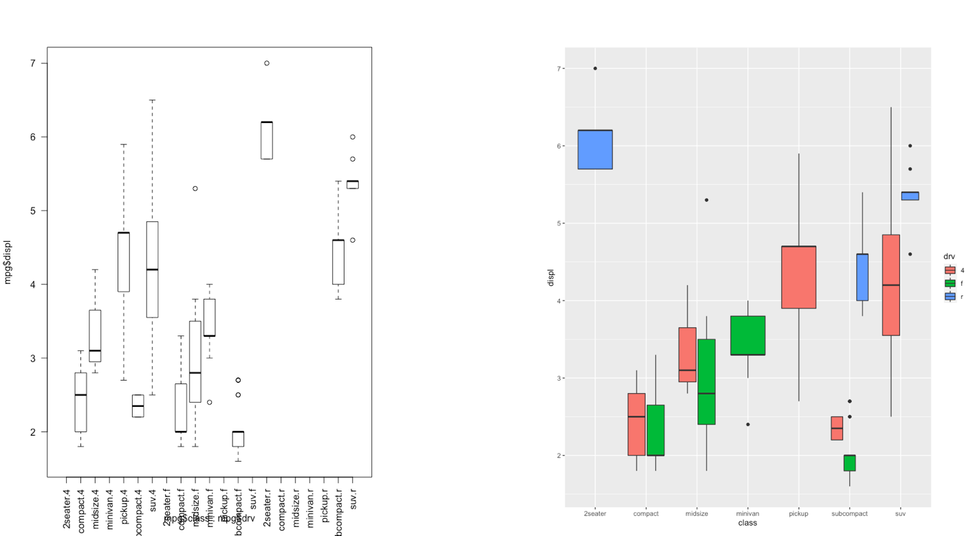
Figure 5.6: Comparison between standard and ggplot2 plots
With ggplot2 a plot is defined by several layers, as shown in Figure 5.7. The first layer specifies the coordinate system, then we can have several geometries each with an aesthetics specification.
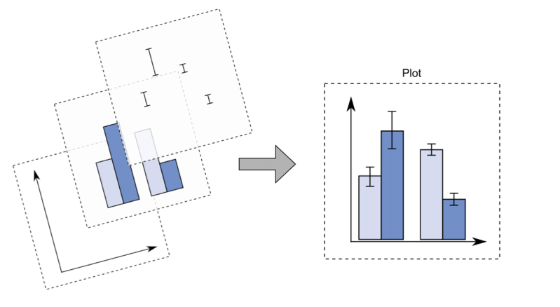
Figure 5.7: The layer structure of the ggplot2 plot
I suggest to download from here the ggplot2 cheat sheet.
The most important function of the ggplot2 library is the ggplot function.
All ggplot plots begin with a call to ggplot supplying the data:
ggplot(data = …) +
  geom_function(mapping = aes(…))
where geom_function is a generic function for a geometry layer; see here for the list of all the available geometries.
For starting a new empty plot we can proceed by using the following code:
prices %>%
  ggplot()
To add components and layers to the empty plot we will use the + symbol (not the pipe).
5.6 Time series plot
A time series plot displays on the x-axis the dates and on the y-axis the values of the prices. A line will connect values, for this reason the geometry we need is called geom_line:
prices %>%
ggplot() +
geom_line(aes(x=DateOK, y=GME))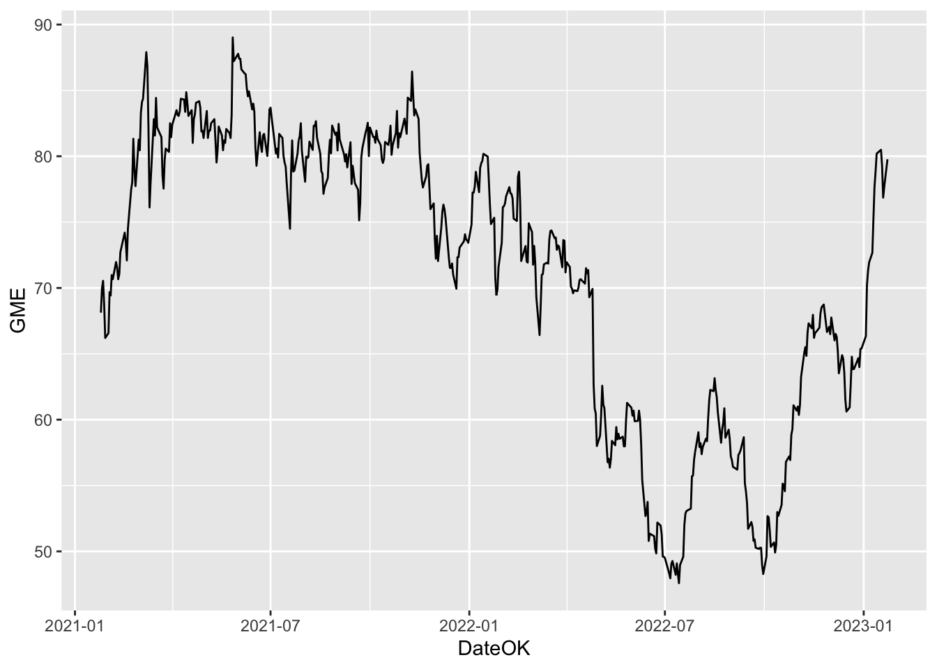 The aesthetic, created by
 aes, describes the visual characteristics that represent the data, e.g. position, size, color, shape, transparency, fill, etc. It is also possible to specify a color for the line (for example blue) as follows:
prices %>%
  ggplot() +
  geom_line(aes(x=DateOK, y=GME), col="blue")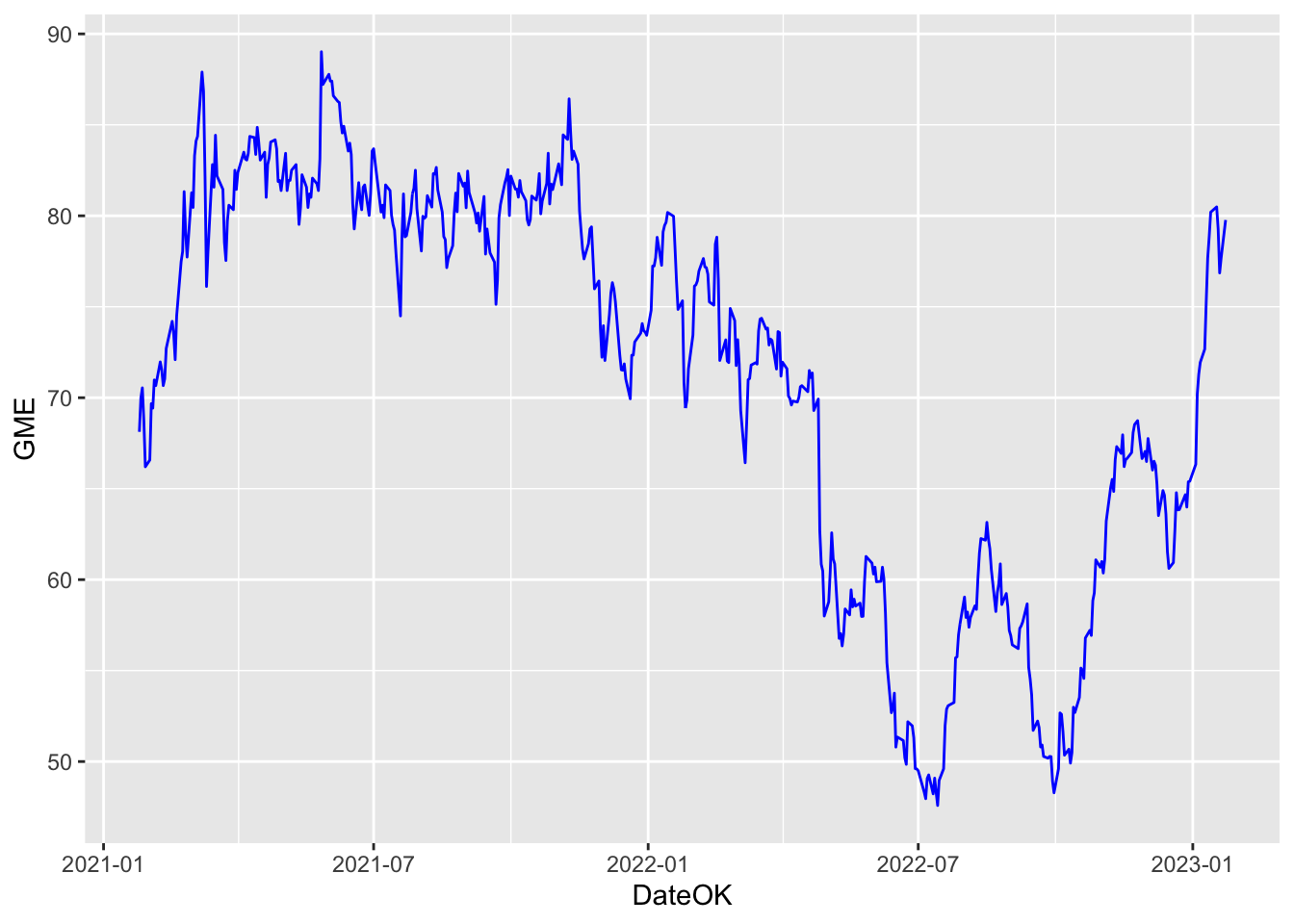
When the color is the same for all the points it is placed outside of aes() and is specified by quotes ("blue"). A different case is when we have a different color for each point according one the variables (for evample GME itself. In this case the color specification is included inside aes():
prices %>%
ggplot() +
geom_line(aes(DateOK, GME, col=GME))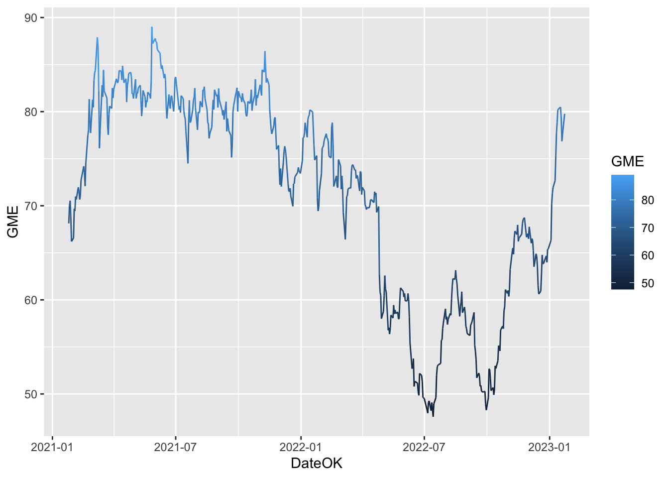 Note that automatically a legend is added that explains the color palette.
5.7 Exercises Lab 3
5.7.1 Exercise 1
Consider the file AdjclosepricesLab3Exercises.csv which is available in the folder Files in the e-learning. It contains the adjusted close prices for 4 assets (Netflix, Amazon, Apple, Tesla).
- Import the data into R and create a new data frame named
p_data. Have a look to the data. How many data do you have?
library(tidyverse)
library(lubridate)
You have a problem with dates. Use the
lubridatepackage and themutateverb to create a new variable with proper dates. Note that the format of the dates is now different (you have day/month/year) and you will need a new function (suggestion:dmy). Which is the considered time period?Create a new variable named
yearwhich contains the year of each observation (use functionyearfrom thelubridatepackage):How many observations in percentage are available for each year? Use
count. Then order the output with respect to the percentage (descending order). Which is the year with the largest percentage of data?Compute the average price for each asset.
Consider now only
NFLX. Compute the average price conditionally onyear. Finally select only the years such that the average price is higher than 410 dollars.Plot the
NFLXtime serie but filtering out the observations before 2019. The color of the time series should be given byyear.