Chapter 12 Lab 10 - 01/06/2023
In this lab we will simulate the SPEF exam which is divided in 3 parts: exploratory data analysis, regression model and time series analysis.
We will use the data contained in the Adjcloseprices9cfu.csv file. It contains the daily adjusted close prices observed from 2017-09-11 to 2021-09-10 for the following assets (data source: Yahoo Finance):
- Apple Inc. (AAPL)
- Globalstar, Inc. (GSAT)
- AMC Entertainment Holdings, Inc. (AMC)
- American Airlines Group Inc. (AAL)
- Ford Motor Company (F)
- NASDAQ Composite (IXIC)
12.1 Part 1: exploratory data analysis
- Import the data in R. Check the dimensions and the structure of the dataframe. If necessary, transform the dates into a proper calendar variable.
library(tidyverse)
prices = read.csv("./files/Adjcloseprices9cfu.csv",sep=";",dec=".",header=TRUE)
dim(prices)
## [1] 1008 7glimpse(prices)## Rows: 1,008
## Columns: 7
## $ Date <chr> "2017-09-11", "2017-09-12", "2017-09-13", "2017-09-14", "2017-09-…
## $ AAPL <dbl> 38.53323, 38.38054, 38.09183, 37.76495, 38.14671, 37.85801, 37.87…
## $ GSAT <dbl> 1.60, 1.68, 1.77, 1.78, 1.82, 1.78, 1.77, 1.80, 1.79, 1.77, 1.72,…
## $ AMC <dbl> 11.32855, 11.40889, 12.21233, 12.89526, 13.61836, 13.37733, 12.57…
## $ AAL <dbl> 44.60053, 45.01872, 45.70923, 44.92147, 44.73669, 44.06564, 43.16…
## $ F <dbl> 9.694755, 9.847696, 9.873184, 9.822205, 9.873184, 9.881683, 9.958…
## $ IXIC <dbl> 6432.26, 6454.28, 6460.19, 6429.08, 6448.47, 6454.64, 6461.32, 64…library(lubridate)
prices$Date = ymd(prices$Date)- Compute the LOG-returns for each price time series.
Here we use the approach described in Section 6 and compute the log-returns in the wide and long version:
# logprices
logprices = prices %>%
  mutate(across(AAPL:IXIC, log))
glimpse(logprices)
## Rows: 1,008
## Columns: 7
## $ Date <date> 2017-09-11, 2017-09-12, 2017-09-13, 2017-09-14, 2017-09-15, 2017…
## $ AAPL <dbl> 3.651521, 3.647550, 3.640000, 3.631382, 3.641440, 3.633843, 3.634…
## $ GSAT <dbl> 0.4700036, 0.5187938, 0.5709795, 0.5766134, 0.5988365, 0.5766134,…
## $ AMC <dbl> 2.427326, 2.434393, 2.502447, 2.556860, 2.611419, 2.593561, 2.531…
## $ AAL <dbl> 3.797746, 3.807078, 3.822300, 3.804916, 3.800794, 3.785680, 3.764…
## $ F <dbl> 2.271585, 2.287238, 2.289822, 2.284646, 2.289822, 2.290683, 2.298…
## $ IXIC <dbl> 8.769081, 8.772499, 8.773414, 8.768587, 8.771598, 8.772555, 8.773…# log-returns
logret = logprices %>%
mutate(across(AAPL : IXIC, ~ . - lag(.)))
glimpse(logret)## Rows: 1,008
## Columns: 7
## $ Date <date> 2017-09-11, 2017-09-12, 2017-09-13, 2017-09-14, 2017-09-15, 2017…
## $ AAPL <dbl> NA, -0.0039706597, -0.0075505803, -0.0086183200, 0.0100580644, -0…
## $ GSAT <dbl> NA, 0.048790164, 0.052185753, 0.005633818, 0.022223137, -0.022223…
## $ AMC <dbl> NA, 0.007067140, 0.068053455, 0.054413451, 0.054558999, -0.017857…
## $ AAL <dbl> NA, 0.0093326603, 0.0152216676, -0.0173841943, -0.0041220400, -0.…
## $ F <dbl> NA, 0.0156525016, 0.0025848759, -0.0051767562, 0.0051767562, 0.00…
## $ IXIC <dbl> NA, 3.417526e-03, 9.152767e-04, -4.827259e-03, 3.011466e-03, 9.56…# remove the first line with na
logret = na.omit(logret)
# from long to wide
logret_long = logret %>%
pivot_longer(AAPL : IXIC)
glimpse(logret_long)## Rows: 6,042
## Columns: 3
## $ Date <date> 2017-09-12, 2017-09-12, 2017-09-12, 2017-09-12, 2017-09-12, 201…
## $ name <chr> "AAPL", "GSAT", "AMC", "AAL", "F", "IXIC", "AAPL", "GSAT", "AMC"…
## $ value <dbl> -0.0039706597, 0.0487901642, 0.0070671399, 0.0093326603, 0.01565…- Provide one single plot containing all the boxplots. Comment the plot discussing the differences between the log-returns distributions.
Here we use the long version of the log-returns dataframe:
logret_long %>%
ggplot() +
geom_boxplot(aes(name, value, fill = name), col = "blue")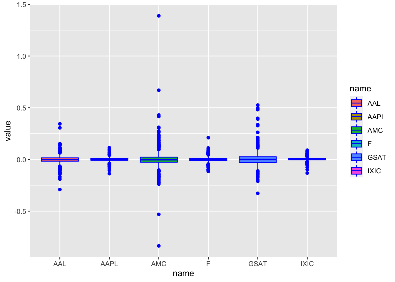 We observe that for all the distributions the median log-return is close to one. Moreover, highly extreme values for AMC and GSAT are visible giving rise to higher variability.
- Which is the distribution with the largest percentage of log-returns bigger than 0.5? Provide the corresponding percentages.
Here we make use of the boxplots computed before to observe that ONLY AMC and GSAT took values bigger than 0.5 so I need to compute only 2 percentages:
mean(logret$AMC>0.5)*100## [1] 0.1986097mean(logret$GSAT>0.5)*100## [1] 0.09930487# AMC has the largest %- Consider the series of
AAPLlog-returns. Provide the normal probability plot. Comment the plot.
qqnorm(logret$AAPL,datax = T)
qqline(logret$AAPL,datax = T)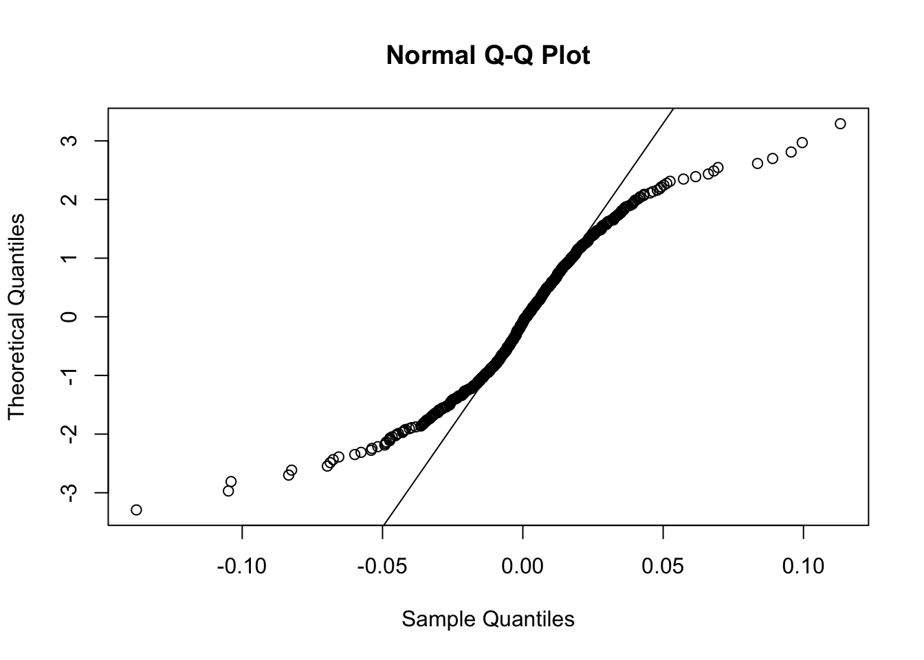 The plot is characterized by a convex-concave pattern which suggest a heavy-tail distribution.
- In order to check the normality of the
AAPLlog-returns distribution, perform a statistical test of your choice; provide the test output and comment the result (\(\alpha\)=0.05).
shapiro.test(logret$AAPL)##
## Shapiro-Wilk normality test
##
## data: logret$AAPL
## W = 0.92463, p-value < 2.2e-16Given the tiny p-value of the Shapiro test, we reject the null hypothesis of normality.
12.2 Part 2: regression analysis
- Consider the log-returns of ALL the variables. Provide the scatterplot matrix. Which is the pair of variables showing tail dependence? Why? Which is the pair of variables showing tail independence? Explain why.
library(GGally)
logret %>%
  dplyr::select(-Date) %>%
  ggpairs()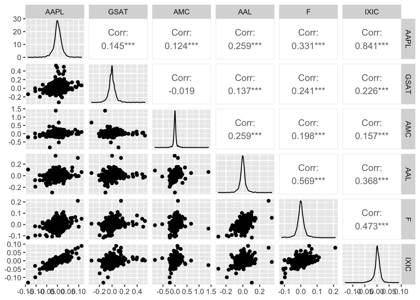
IXIC and AAPL are positively correlated and show tail-dependence (extremely low or high values of their log-returns occur jointly). An example of tail-independence is given by GSAT and AMC: when we observe extremely high values of GSAT we don’t have also extremely high values of AMC which are instead close to zero.
- Estimate the multiple regression model using the
IXIClog-returns as dependent variable and, as independent variables, the remaining log-returns series. Provide the summary for the full regression model.
mod1 = lm(IXIC ~. -Date, logret)
summary(mod1)
##
## Call:
## lm(formula = IXIC ~ . - Date, data = logret)
##
## Residuals:
## Min 1Q Median 3Q Max
## -0.044398 -0.003790 0.000146 0.004033 0.035869
##
## Coefficients:
## Estimate Std. Error t value Pr(>|t|)
## (Intercept) 9.799e-05 2.312e-04 0.424 0.671702
## AAPL 5.459e-01 1.198e-02 45.582 < 2e-16 ***
## GSAT 1.553e-02 3.700e-03 4.199 2.93e-05 ***
## AMC 2.464e-03 2.827e-03 0.872 0.383549
## AAL 2.484e-02 7.439e-03 3.339 0.000872 ***
## F 1.028e-01 1.220e-02 8.425 < 2e-16 ***
## ---
## Signif. codes: 0 '***' 0.001 '**' 0.01 '*' 0.05 '.' 0.1 ' ' 1
##
## Residual standard error: 0.007312 on 1001 degrees of freedom
## Multiple R-squared: 0.7576, Adjusted R-squared: 0.7564
## F-statistic: 625.6 on 5 and 1001 DF, p-value: < 2.2e-16- Discuss the significance of the coefficients (\(\alpha\) = 0.05), specifying which is the null hypothesis you are testing. Do you think that any regressor should be removed? If yes, remove, one by one, the regressor(s) and provide the summary of the final reduced model.
From the previous summary table we can use the t-tests to verify if each regressor coefficient is significantly different from zero. Given the high p-value of AMC we conclude that its beta coefficient is not significantly different from zero and it does not exist a significant linear relationship with IXIC. For this reason we remove the regressor.
mod2 = lm(IXIC ~. -Date - AMC, logret)
summary(mod2)
##
## Call:
## lm(formula = IXIC ~ . - Date - AMC, data = logret)
##
## Residuals:
## Min 1Q Median 3Q Max
## -0.044927 -0.003801 0.000150 0.004086 0.035774
##
## Coefficients:
## Estimate Std. Error t value Pr(>|t|)
## (Intercept) 0.0001018 0.0002311 0.441 0.659668
## AAPL 0.5464533 0.0119576 45.699 < 2e-16 ***
## GSAT 0.0152934 0.0036892 4.145 3.68e-05 ***
## AAL 0.0259799 0.0073213 3.549 0.000405 ***
## F 0.1034725 0.0121738 8.500 < 2e-16 ***
## ---
## Signif. codes: 0 '***' 0.001 '**' 0.01 '*' 0.05 '.' 0.1 ' ' 1
##
## Residual standard error: 0.007311 on 1002 degrees of freedom
## Multiple R-squared: 0.7574, Adjusted R-squared: 0.7564
## F-statistic: 782.1 on 4 and 1002 DF, p-value: < 2.2e-16With the reduced model all the coefficients are significantly different from zero and the goodness of fit is basically unchanged.
- Discuss the goodness of fit of the final model obtained at the previous point (to be considered from here onward). What can you conclude?
The goodness of fit given by the R-squared is equal to 0.75: the 75% of the variability of IXIC is explained by the regressors.
- Provide the plot of the Cook’s distance. Compute the percentage of influential cases.
data.frame(
  index = 1:nrow(logret),
  cooks = cooks.distance(mod2)) %>%
  ggplot() +
  geom_point(aes(index,cooks)) +
  geom_text(aes(index,cooks, label=index),nudge_y = 0.005) +
  geom_hline(yintercept=4/nrow(logret),col="red")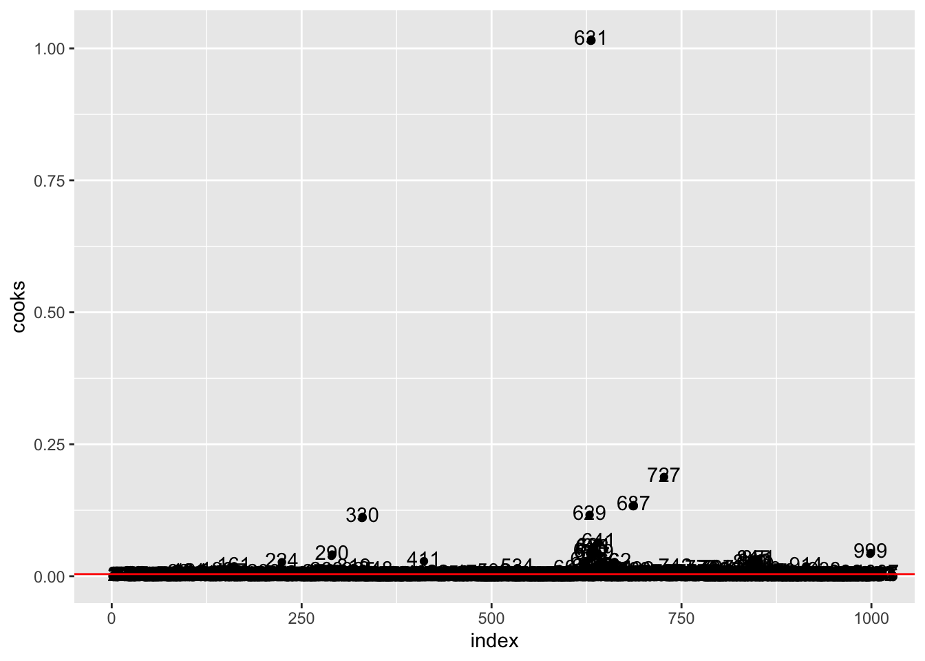
mean(cooks.distance(mod2) > 4/nrow(logret))*100## [1] 7.249255logret[631,]## Date AAPL GSAT AMC AAL F IXIC
## 632 2020-03-16 -0.137708 -0.1381503 -0.2138699 0.1066176 -0.1166735 -0.1314915We percentage of influential cases is about 7%. In particular observation n. 631, with the highest values of the Cook’s distance, is the most influential case.
- Consider the raw residuals of your final model and check the homoscedasticity assumption. Provide the necessary plot and comment it.
data.frame(fitted = mod2$fitted.values,
  res = mod2$residuals) %>%
  ggplot(aes(fitted,abs(res))) +
  geom_point() +
  geom_smooth()
## `geom_smooth()` using method = 'gam' and formula 'y ~ s(x, bs = "cs")'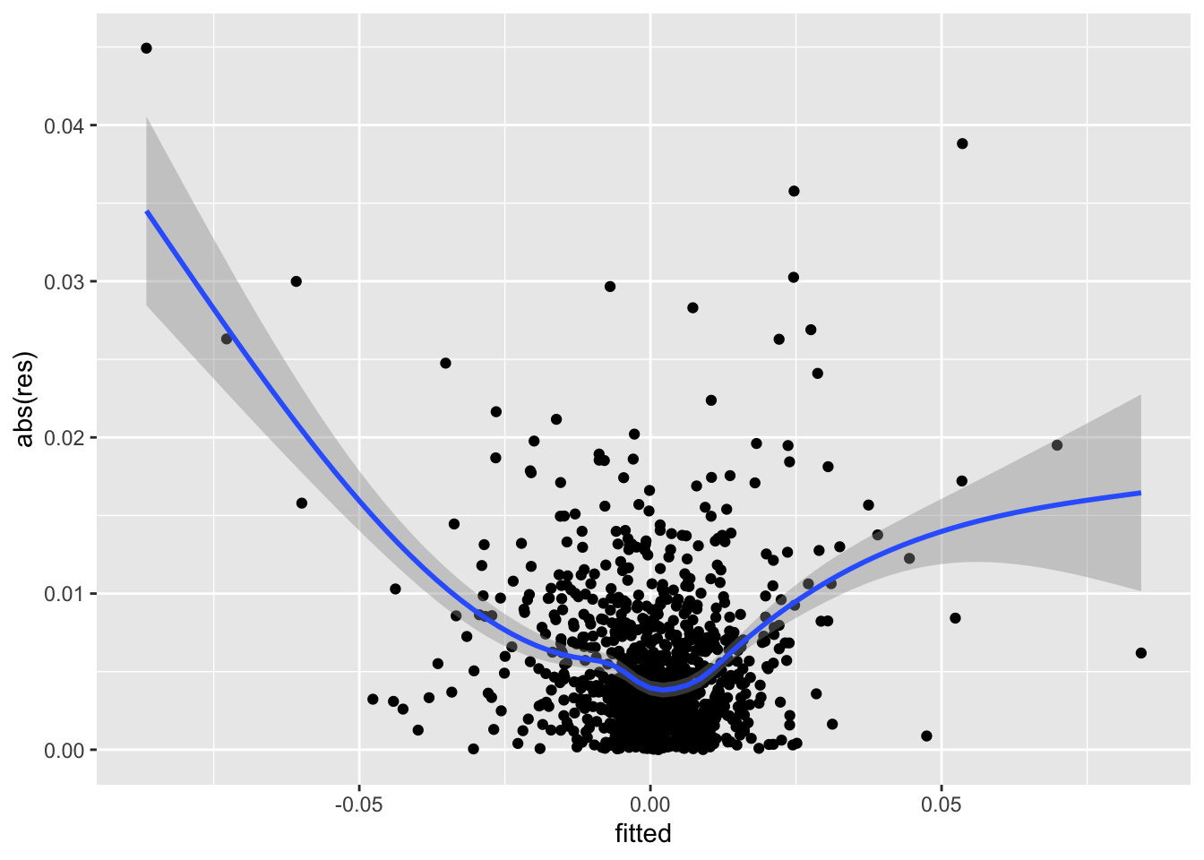 Given the u-shape pattern we observe in the plot, we conclude that the homoschedasticity assumption should be rejected.
- Given the final regression model, plot the observed and predicted values of the response variable. Comment the plot.
data.frame(obs = logret$IXIC,
           pred = mod2$fitted.values) %>%
  ggplot(aes(obs,pred)) +
  geom_point() +
  geom_abline(slope = 1, intercept = 0)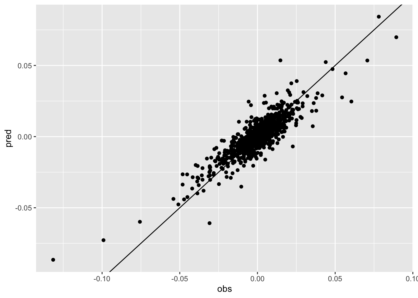
cor(logret$IXIC,mod2$fitted.values)## [1] 0.8702864The correlation between observed and predicted values is equal to 0.87 as showed by the cloud of points which is pretty aligned along the bisector line.
12.3 Part 3: time series analysis and ARMA models
Consider the AMC log-returns.
- Provide the time series plot of the
AMClog-returns. Comment about the stationarity and volatility of the time series.
logret %>%
ggplot()+
geom_line(aes(Date, AMC))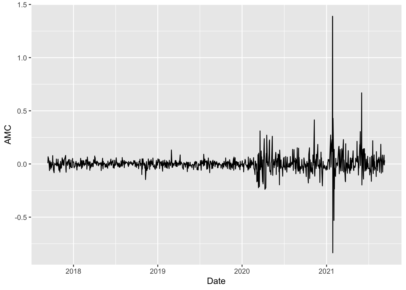 We observe that the time-series is mean reverting but is not stationary with respect to the variance which is increasing in time especially after 2020.
- Provide the plot of the autocorrelation function (ACF). Comment the plot.
The plot of the auto-correlation function, known as correlogram, can be obtained by using the same function acf
acf(logret$AMC)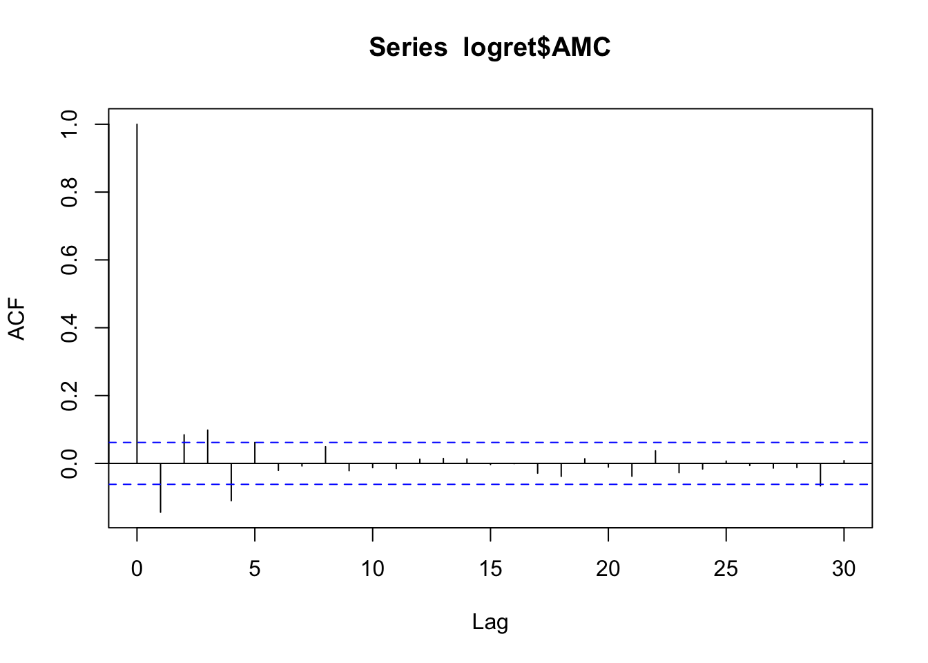 The vertical bars for the lags from 1 to 4 are outside from the blue lines; this means that the autocorrelation at these lags is significantly different from zero (so there is temporal correlation in the series). For the following lags the vertical bars are contained between the blue lines. This means that from lag 5 onward there are no significant correlations. We wonder the pattern we observe could resemble a well-known ARMA model. Given that we have only the first 4 correlations to be different from zero, this could remind us of a cut-off behavior typical of MA models. We thus check if, as expected, the partial autocorrelation plot is characterized by a tail-off behavior:
pacf(logret$AMC)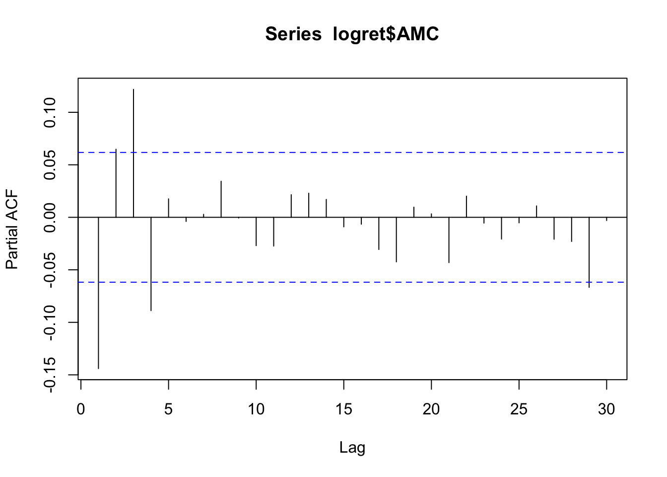
Unfortunately, the PACF plot, which starts with \(h=1\), doesn’t show a clear tail-off pattern.
- Estimate the following ARMA models for the
AMClog-returns: AR(1), AR(2), AR(3), MA(1), MA(2), MA(3). Which are the best and the worst model for describing the temporal pattern of the data? Why?
We will use the Arima function which is part of the forecast package. For estimating a model, we have to specify the data and the order \((p,d,q)\) of the model. It is known that the Arima function adopts maximum likelihood for estimation; thus, the coefficients are asymptotically normally distributed. Hence, if you the divide each coefficient by its standard error you get the corresponding z-statistic value and it is then possible to compute the p-value to test if the parameter is significantly different from zero. For comparing the models we will use the AIC index (the lower the better):
library(forecast)## Registered S3 method overwritten by 'quantmod':
## method from
## as.zoo.data.frame zoomodAR1 = Arima(logret$AMC, order=c(1,0,0))
modAR1## Series: logret$AMC
## ARIMA(1,0,0) with non-zero mean
##
## Coefficients:
## ar1 mean
## -0.1439 0.0015
## s.e. 0.0312 0.0023
##
## sigma^2 = 0.00707: log likelihood = 1065.38
## AIC=-2124.77 AICc=-2124.75 BIC=-2110.03modAR1$aic## [1] -2124.769modAR2 = Arima(logret$AMC, order=c(2,0,0))
modAR2## Series: logret$AMC
## ARIMA(2,0,0) with non-zero mean
##
## Coefficients:
## ar1 ar2 mean
## -0.1345 0.0647 0.0015
## s.e. 0.0314 0.0314 0.0025
##
## sigma^2 = 0.007048: log likelihood = 1067.5
## AIC=-2127 AICc=-2126.96 BIC=-2107.34modAR2$aic## [1] -2126.999modAR3 = Arima(logret$AMC, order=c(3,0,0))
modAR3## Series: logret$AMC
## ARIMA(3,0,0) with non-zero mean
##
## Coefficients:
## ar1 ar2 ar3 mean
## -0.1424 0.0812 0.1217 0.0015
## s.e. 0.0313 0.0315 0.0312 0.0028
##
## sigma^2 = 0.00695: log likelihood = 1075.02
## AIC=-2140.04 AICc=-2139.98 BIC=-2115.46modAR3$aic## [1] -2140.038modMA1 = Arima(logret$AMC, order=c(0,0,1))
modMA1## Series: logret$AMC
## ARIMA(0,0,1) with non-zero mean
##
## Coefficients:
## ma1 mean
## -0.1219 0.0015
## s.e. 0.0282 0.0023
##
## sigma^2 = 0.007092: log likelihood = 1063.83
## AIC=-2121.66 AICc=-2121.63 BIC=-2106.91modMA1$aic## [1] -2121.657modMA2 = Arima(logret$AMC, order=c(0,0,2))
modMA2## Series: logret$AMC
## ARIMA(0,0,2) with non-zero mean
##
## Coefficients:
## ma1 ma2 mean
## -0.1507 0.1325 0.0015
## s.e. 0.0313 0.0343 0.0026
##
## sigma^2 = 0.006999: log likelihood = 1070.97
## AIC=-2133.94 AICc=-2133.9 BIC=-2114.28modMA2$aic## [1] -2133.941modMA3 = Arima(logret$AMC, order=c(0,0,3))
modMA3## Series: logret$AMC
## ARIMA(0,0,3) with non-zero mean
##
## Coefficients:
## ma1 ma2 ma3 mean
## -0.1301 0.1141 0.0672 0.0015
## s.e. 0.0326 0.0353 0.0337 0.0028
##
## sigma^2 = 0.006978: log likelihood = 1072.94
## AIC=-2135.88 AICc=-2135.82 BIC=-2111.31modMA3$aic## [1] -2135.885The model with the lowest AIC value is AR(3). We now study its residuals in order to see if there is still some temporal correlation left. We can use the checkresiduals function from the forecast package which provides some plots for the residuals (i.e. the time-series plot and the correlogram) and the simultaneous Ljung-Box test output.
checkresiduals(modAR3)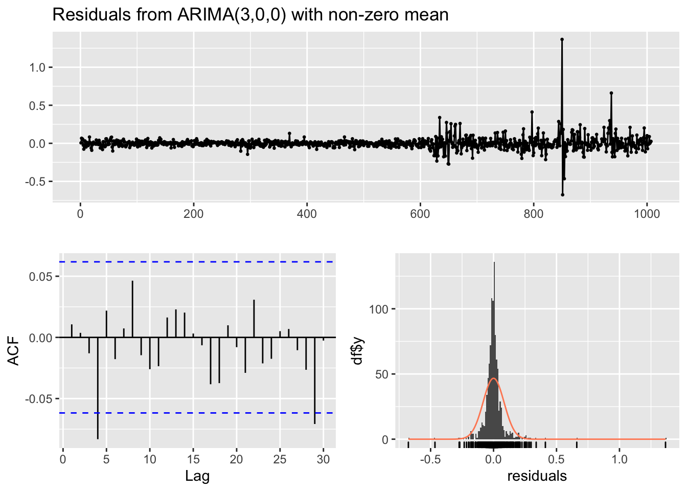
##
##  Ljung-Box test
##
## data:  Residuals from ARIMA(3,0,0) with non-zero mean
## Q* = 11.263, df = 6, p-value = 0.08057
##
## Model df: 4.   Total lags used: 10
Note that in the Ljung-Box test (given in the Console) the number of considered lags is 10 (Total lags used). This means that we are checking if the first 10 correlations are jointly equal to zero; if necessary this can be changed by using the lag argument (in this case for example we can just focus on the first 5 lags, see the ACF plot). Moreover, the number of model degrees of freedom is 4 (given by the number of parameters estimated with the AR3 model, mean included) and the number of degrees of freedom of the \(\chi^2\) distribution is 10-4=6.
checkresiduals(modAR3, lag=5)
##
##  Ljung-Box test
##
## data:  Residuals from ARIMA(3,0,0) with non-zero mean
## Q* = 7.7987, df = 1, p-value = 0.005228
##
## Model df: 4.   Total lags used: 5
Given the p-value we reject the simultaneous uncorrelation hypothesis of the first 5 autocorrelations (in particular the one at lag 4 is significantly different from zero). It means that the AR(3) is not enough for catching the temporal structure of the data.
We can use the auto.arima function from the forecast package to have an automatic estimation of the best ARMA model over many possible models:
auto1 = auto.arima(logret$AMC)
auto1
## Series: logret$AMC
## ARIMA(4,0,0) with zero mean
##
## Coefficients:
## ar1 ar2 ar3 ar4
## -0.1313 0.0887 0.1093 -0.0883
## s.e. 0.0314 0.0315 0.0314 0.0314
##
## sigma^2 = 0.006897: log likelihood = 1078.82
## AIC=-2147.65 AICc=-2147.59 BIC=-2123.07checkresiduals(auto1)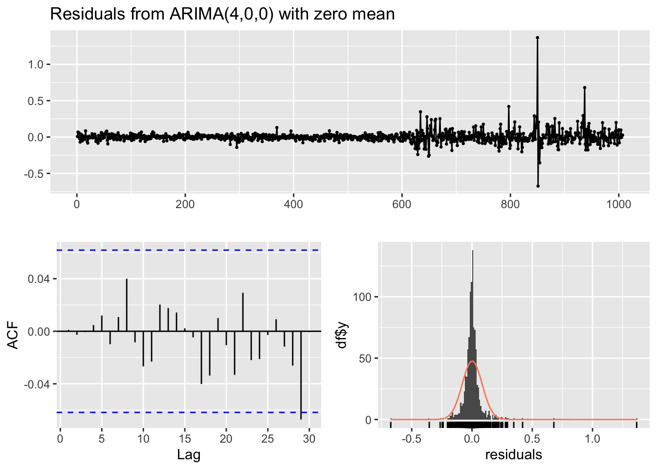
##
##  Ljung-Box test
##
## data:  Residuals from ARIMA(4,0,0) with zero mean
## Q* = 2.821, df = 6, p-value = 0.831
##
## Model df: 4.   Total lags used: 10
It results that the AR(4) model is the best one (again in terms of AIC). Also the ACF plot and the Ljung-Box test output (for \(h=10\)) show that there is not residual correlation (there is a vertical bar at lag 29 in the ACF which is out of the blue bar but we shouldn’t care about it).
Given that the residuals are not correlated we can perform forecasting of the log-returns. To do this we use the forecast function:
forecast(auto1)## Point Forecast Lo 80 Hi 80 Lo 95 Hi 95
## 1008 -1.061442e-02 -0.11704594 0.09581709 -0.1733874 0.1521585
## 1009 7.690417e-03 -0.09965481 0.11503565 -0.1564799 0.1718608
## 1010 -3.822189e-04 -0.10831760 0.10755316 -0.1654551 0.1646907
## 1011 -3.364294e-03 -0.11166672 0.10493814 -0.1689986 0.1622700
## 1012 2.185813e-03 -0.10668394 0.11105557 -0.1643161 0.1686877
## 1013 -1.306457e-03 -0.11027820 0.10766529 -0.1679644 0.1653514
## 1014 3.155204e-05 -0.10895232 0.10901542 -0.1666449 0.1667080
## 1015 4.160451e-04 -0.10857641 0.10940850 -0.1662735 0.1671056
## 1016 -3.876719e-04 -0.10939088 0.10861554 -0.1670937 0.1663184
## 1017 2.066561e-04 -0.10880041 0.10921372 -0.1665053 0.1669186The output table contains the point forecasts and the extreme of the prediction intervals with \(1-\alpha\) equal to 0.80 and 0.95. The corresponding plot is given by
forecast(auto1) %>%
autoplot()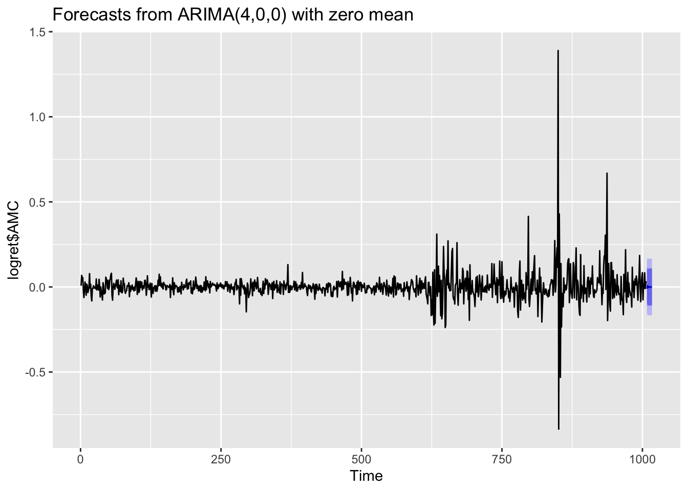 If you are interested in obtaining more forecasts, you can use use the
 h option:
forecast(auto1, h=50) %>%
autoplot()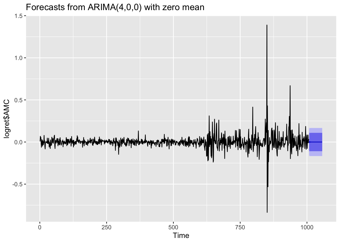 As expected for stationary models, the \(k\)-step forecast \(\hat y_{n+k}\) converges to the estimated mean \(\hat \mu\) as \(k\rightarrow +\infty\). Moreover, the \(k\)-step forecast error converges to a finite value as \(k\rightarrow +\infty\) and the forecast bounds converge to parallel horizontal lines. The limitation of the plot is that it doesn’t use calendar dates in the horizontal axis and we should need some extra code to fix this.
12.4 Exercise Lab 10
The text of the exercises are available in the file R_Lab10_exercises.Rmd
file (available in fhte Files folder of the Moodle page). Use this file to run your code for solving the exercises. Include also your
comments. Check step by step your html output in the RStudio Viewer pane.