Chapter 3 Lab 1 - 28/02/2023
In this lab we will learn the basic commands for programming with R. We will work in RStudio.
Place your cursor in the Console and type the following code or any other mathematical operation:
5+4## [1] 9R can work like a calculator and you can compute whatever quantity you need. The point is that if you close RStudio, you will lose all your code. To avoid this, I suggest to use scripts (i.e. text files where you can write and run your code). To open a new one, use the RStudio menu: File - New File - RScript. Write all your code in your script(s) and use ctrl/cmd + enter to run the code in the Console. Save the script by using the menu: File - Save as…. The extension of a script is .R (choose the name you prefer). In the future you will be able to open your script with RStudio (File - Open File) without losing any code.
3.1 Built-in functions
Before starting using a function, it is good practice to visualise the help page (by running ?nameofthefunction), in order to understand how the function is defined and which are its arguments and the default settings.
To run a function (and get the results) type the name of the function followed by round parentheses, inside which you specify the arguments of the functions (the inputs).
For example to compute the logarithm of a number the function log is used. Its help page can be obtained by
?logNote that the function is characterized by two arguments (inputs): x (number/vector for which the log is computed) and base (the base of the log function, by default it’s the natural log).
Let’s compute the log as follows:
log(x = 5 , base = 10) #log of 5 with base 10## [1] 0.69897log(x = 5) #natural log ## [1] 1.609438Argument names can be omitted. In this case it is very important to be careful about the order of the arguments passed to the function (the order is given by the function definition, check the help).
log(5, 10)## [1] 0.69897log(10, 5) #warning: this is log of 10 with base 5## [1] 1.4306773.2 Objects and vectors
In R it is possible to create objects by using the assignment operator = (it is also possible to use <-). As argument name you can choose any name you prefer; however, it’s better to use short and meaningful names. The following code assigns the number -1.5 to the object named w (have a look to the top right panel!):
w = -1.5A vector of number is created using the c function (concatenate). For example the following code is used to create a vector with 4 numbers. The vector is saved in an object named x:
x = c(-5, log(4), exp(6), 10^4, -0.5)
x
## [1] -5.000000 1.386294 403.428793 10000.000000 -0.500000It is also possible to create a new vector y by transforming x (element by element):
y = x - 1The output y is a new vector,
To visualize the values of y just run the object name (remember that R is case-sensitive so that y is different from Y):
y## [1] -6.0000000 0.3862944 402.4287935 9999.0000000 -1.5000000The vector length is given by
length(y)## [1] 5It is possible to compute operations with vectors (of the same length). For example, the following code
x + y ## [1] -11.000000 1.772589 805.857587 19999.000000 -2.000000add each value of x to the corresponding value of y. Note that R executes operations with vector element-wise (element by element singularly).
It is also possible to summarize the values in a vector by using summary statistics function such as the sum or the mean applied to x or any function of it:
min(x)## [1] -5max(x)## [1] 10000sum(x) #sum of the elements of y## [1] 10399.32mean(x) #mean of the values of y## [1] 2079.863sum(x) / length(x) #another way for computing the mean## [1] 2079.863median(x)## [1] 1.386294quantile(x)## 0% 25% 50% 75% 100%
## -5.000000 -0.500000 1.386294 403.428793 10000.000000var(x)## [1] 19633408mean((x^3)+4) ## [1] 200013131973Note that we have two (or more) nested functions (like in the latter case) they are executed from the inside to the outside (first the operation \(^3+4\) is computed and then the sum).
To select elements from a vector we use squared parentheses. For example, to retrieve the second element the following code is used, where inside the parentheses the position of the element to be select is specified:
x[1] ## [1] -5To select more than one element, a vector of positions is provided:
x[c(1,5)] #select the first and last element## [1] -5.0 -0.5x[c(1,length(x))] #equivalent code## [1] -5.0 -0.5If you need to select the first four element of y you can proceed as follows:
x[c(1,2,3,4)]## [1] -5.000000 1.386294 403.428793 10000.000000or by using the following shorter code where 1:4 generates a regular sequence of integers from 1 to 4:
1:4## [1] 1 2 3 4x[1:4]## [1] -5.000000 1.386294 403.428793 10000.000000It is also possible to compute logical operation whose result is TRUE if the condition is met or FALSE otherwise. For example we want to check if the elements of x are negative:
x < 0## [1] TRUE FALSE FALSE FALSE TRUEThis returns a vector of TRUE/FALSE according to the condition x<0 applied to each element of x. Summary statistics can be applied also to vector of logical values, in this case TRUE is considered as 1 and FALSE as 0.
sum(x < 0) #number of values < 0 ## [1] 2mean(x < 0) #proportion of values < 0## [1] 0.4mean(x < 0)*100 #% of values < 0## [1] 40The following table lists all the logical operators available in R.
| Operator in R | Description |
|---|---|
| <= >= | lower/bigger than or equal |
| < > | lower/bigger |
| == | exactly equal to |
| != | different from |
| & | intersection (and) |
| (vertical bar) |
union (or) |
By using logical operator it is possible to select/replace elements in a vector by setting a condition. In this case it is not necessary to specify the positions in the vector of the elements to be selected/replaced. R will consider only the elements for which the condition is met:
# substitute the negative numbers of x with 0
x[x > 0] = 0
x
## [1] -5.0 0.0 0.0 0.0 -0.5Let’s create now a new vector object called x2 which contains all the element of x different from -5 In this case the condition which is tested is z == -5 which returns
x == -5## [1] TRUE FALSE FALSE FALSE FALSEbut we are instead interested in the complementary condition which can be obtained by using the exclamation mark in two possible ways:
! (x == -5)## [1] FALSE TRUE TRUE TRUE TRUEx != -5## [1] FALSE TRUE TRUE TRUE TRUEFinally, we can do the selection and create x2:
x2 = x[! x == -5]
x2
## [1] 0.0 0.0 0.0 -0.53.3 Simulation of values from a model
Let’s consider the following model involving one quantitative regressor \(X\) and a quantitative response variable \(Y\): \[ Y = f(X) + \epsilon \] where \[ f(X)=sin(1.3x)15 + 3(x - 4)^2 \] and \(\epsilon\) is distributed like a Normal distribution with mean equal to 0 and variance 100.
In R by start by setting the \(x\) values. In particular we consider a regular sequence from 0 to 12 of length 50 created by using the function seq (see ?seq):
xseq = seq(from = 0,
           to = 12,
           length = 50)
xseq
## [1] 0.0000000 0.2448980 0.4897959 0.7346939 0.9795918 1.2244898
## [7] 1.4693878 1.7142857 1.9591837 2.2040816 2.4489796 2.6938776
## [13] 2.9387755 3.1836735 3.4285714 3.6734694 3.9183673 4.1632653
## [19] 4.4081633 4.6530612 4.8979592 5.1428571 5.3877551 5.6326531
## [25] 5.8775510 6.1224490 6.3673469 6.6122449 6.8571429 7.1020408
## [31] 7.3469388 7.5918367 7.8367347 8.0816327 8.3265306 8.5714286
## [37] 8.8163265 9.0612245 9.3061224 9.5510204 9.7959184 10.0408163
## [43] 10.2857143 10.5306122 10.7755102 11.0204082 11.2653061 11.5102041
## [49] 11.7551020 12.0000000Then we apply the \(f(X)\) defined above as follows:
f = sin(1.3 * xseq)*15 + 3*(xseq - 4)^2This will give rise to a new vector f of length 50.
We now simulate randomly the values for \(\epsilon\) from a Normal distribution. We will use the rnorm function (see ?rnorm):
eps = rnorm(n = 50, mean = 0, sd = sqrt(100))Note that the values in eps are random and will be different every time the code is run (they rare randomly generated!).
We finally sum the values of \(f(X)\) with the values of \(\epsilon\) in order to get \(Y\):
y = f + epsThis will be a new vector of length 50. We now plot the data:
plot(xseq, f, col="red")
points(xseq, y, col="blue")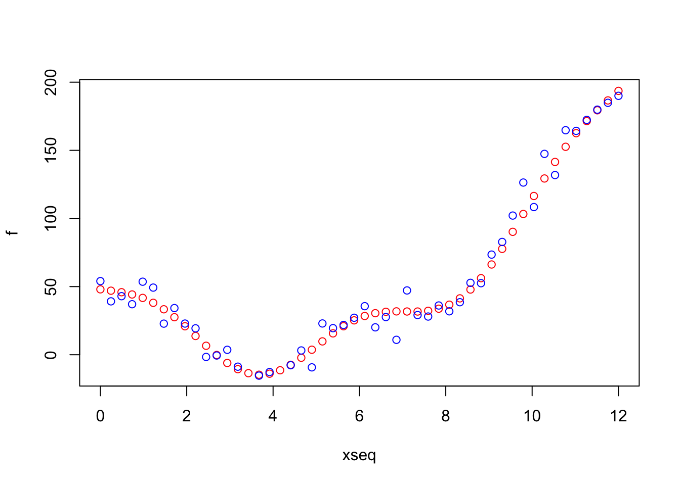 The function
 plot creates the graphical device while points adds some points to an already existing graphical window (remember that your blue points will be different!). The red points represent the true function \(f\) while the blue points are the training data which include some random variation given by \(\epsilon\).
3.4 Data frame
In R a data frame is a matrix which can contain both quantitative and categorical variables. We create a data frame which includes xseq, f and y (for 50 observations):
df = data.frame(xseq, f, y)It is possibile to retrieve the dimensions of the bivariate object and its structure:
dim(df)## [1] 50 3str(df)## 'data.frame': 50 obs. of 3 variables:
## $ xseq: num 0 0.245 0.49 0.735 0.98 ...
## $ f : num 48 47 45.9 44.2 41.7 ...
## $ y : num 54 39.2 43 37.1 53.6 ...Using squared parentheses it is possible to perform data extraction. Given that the data frame object is bidimensional it is necessary to specify two indexes ([row index, column index]). The following code for example extracts the value in the first row, third column:
df[1, 3] ## [1] 54.02375If we omit one of the two indexes we will select a specific row or column:
df[1, ] # one row, all the columns## xseq f y
## 1 0 48 54.02375df[ , 3] # all the rows, one column## [1] 54.0237464 39.1782408 42.9660478 37.0798636 53.5993062 49.2768445
## [7] 22.8276089 34.2433962 22.8856973 19.3827589 -1.6155789 -0.5707967
## [13] 3.6195207 -8.7485469 -27.1332055 -15.3438862 -12.7027526 -34.9541680
## [19] -7.7112013 3.1464562 -9.2585097 22.9561464 19.5223659 21.8786648
## [25] 27.1512190 35.6364995 20.1120544 27.6502928 10.9550525 47.1815372
## [31] 29.1285819 28.0313932 36.1470733 31.8592127 38.5465115 52.7782004
## [37] 52.5075083 73.4917971 82.7726526 102.1331242 126.3670433 108.3626141
## [43] 147.4043136 131.8588825 164.7707637 164.2771731 172.3475909 179.8637527
## [49] 184.8688903 189.9986337When selecting a column (i.e. a variable) it is also possible to select it by name instead that by index. The following code for example select the variable named y:
df$y## [1] 54.0237464 39.1782408 42.9660478 37.0798636 53.5993062 49.2768445
## [7] 22.8276089 34.2433962 22.8856973 19.3827589 -1.6155789 -0.5707967
## [13] 3.6195207 -8.7485469 -27.1332055 -15.3438862 -12.7027526 -34.9541680
## [19] -7.7112013 3.1464562 -9.2585097 22.9561464 19.5223659 21.8786648
## [25] 27.1512190 35.6364995 20.1120544 27.6502928 10.9550525 47.1815372
## [31] 29.1285819 28.0313932 36.1470733 31.8592127 38.5465115 52.7782004
## [37] 52.5075083 73.4917971 82.7726526 102.1331242 126.3670433 108.3626141
## [43] 147.4043136 131.8588825 164.7707637 164.2771731 172.3475909 179.8637527
## [49] 184.8688903 189.99863373.5 Exercises Lab 1
3.5.1 Exercise 1
Compute \(\exp(3-\frac{4}{5})+\frac{\sqrt{3+2^5}}{4-7\cdot \log(10))}\)
Create the vector named
xwhich contains the following values \((10, log(0.2), 6/7, exp(4), sqrt(54), -0.124)\):
- Find the length of
x. - Which elements of of
xare between 0 (included) AND 1 (excluded)? Hint: the AND operator is given by&. Compute also the corresponding absolute (count) and relative frequency (proportions). - Which elements of
xare negative? Substitute them with the same number in absolute value. - Extract from
xthe 2nd and 4th value and save them in a new vector namedy. Compute \(y+sqrt(exp(-0.4))\).
3.5.2 Exercise 2
- Read the help pages of the functions
sampleandseq.
?sample
?seq- Run the following lines of code and try to understand what it is going on.
#Attention: we set the seed in order to work with the same data
set.seed(2233)
xVec = sample(seq(0,999), 25, replace=T)
xVec
## [1] 513 773 693 506 706 208 111 713 816 773 465 661 561 883 871 158 498 91 95
## [20] 94 685 564 833 746 425set.seed(3344)
yVec = sample(seq(0,999, length=100), 25, replace=F)
yVec## [1] 908.18182 888.00000 999.00000 40.36364 433.90909 938.45455 615.54545
## [8] 898.09091 363.27273 817.36364 736.63636 494.45455 242.18182 948.54545
## [15] 302.72727 181.63636 807.27273 555.00000 353.18182 464.18182 797.18182
## [22] 222.00000 766.90909 988.90909 696.27273set.seed(33)
zVec = sample(seq(0,999, by=10), 5, replace=F)
zVec## [1] 410 70 850 590 80Compute some summary statistics for the three vectors.
Select the values in
yVecwhich are bigger than 600.Select the values in
yVecwhich are between 600 and 800 and save them in a new vector calledyVec_sel1. Pick out the values inyVecwhich are bigger than 600 or lower than 800 and save them in a new vector calledyVec_sel2. Which is the length ofyVec_sel1andyVec_sel2?Which are the values in
xVecthat correspond to the values inyVecwhich are bigger than 600? (By correspond, I mean that they have the same positions).Compute the sum and the difference of the first 5 elements of the 2 vectors. Hint: to index the first 5 elements you can use
1:5.For
xVeccompute the following formula \(\frac{\sum_{i=1}^n (x_i-\bar x)^2}{n}\), where \(n\) is the vector length and \(\bar x\) is the vector mean. Is the result equal to the one obtained withvar? Why?For
xVeccompute the following formula \(\frac{\sum_{i=1}^n |x_i-Me|}{n}\), where \(n\) is the vector length and \(Me\) is the vector median.
3.5.3 Exercise 3
Consider the following model \[ Y = \beta_0+\beta_1X +\epsilon \] where \(\beta_0=2\), \(\beta_1=0.3\) and \(\epsilon\) is a Normal distribution with mean 0 and variance 1. 1. Considering a sequence of values for \(X\) between 0 and 10, simulate 200 values for \(Y\). 2. Plot the simulated values.