Chapter 10 Time Series

This chapter focuses on Time Series methods. The most basic time series data is one where we have a single variable that is observed at multiple points in time. The general goal in time series is to take a data series and decompose it in such a way to separate a time trend, cyclicality, seasonality (usually only in the case of non-annual data), and random noise.

We will be making use of many new libraries in this chapter; make sure you have tseries, dynlm, forecast, Hmisc, collapse, installed before getting much further into this chapter.

As usual, we start with loading some data for use in this chapter from the wooldridge and AER packages:

data(ArgentinaCPI)
data(okun)
data(beveridge)
data(BondYield)
data(FrozenJuice)
data(NYSESW)
data(consump)

10.1 Preparing Time Series Data

Before using time series methods, we need to identify the data we are using as being time series data. Because R treats time series data differently than it does run-of-the-mill data frames, this step is essential, because attempting to use time series functions data not identified as time series will result in error messages.

Only some of the data we are dealing with (the data coming from the AER package) are already declared as time series data. Thus, knowing how to declare data as time series is an essential first step for working with it in R.

To illustrate the steps, I will convert the ArgentinaCPI data already loaded into a vector with the as.numeric(ArgentinaCPI) function:

tempCPI <- as.numeric(ArgentinaCPI)

Now, both ArgentinaCPI and tempCPI exist in my environment: the former as a time series object, the latter as simply a list of numbers. If you inspect them in the environment window, you will see they have slightly different descriptions:

• ArgentinaCPI: Time-Series [1:80] from 1970 to 1990: 1.01, 1.06, …

• tempCPI: num [1:80] 1.01, 1.06, 1.13, …

If you look at the data, they display differently as well:

ArgentinaCPI

##              Qtr1         Qtr2         Qtr3         Qtr4
## 1970 1.010000e+00 1.060000e+00 1.130000e+00 1.240000e+00
## 1971 1.330000e+00 1.450000e+00 1.640000e+00 1.770000e+00
## 1972 2.240000e+00 2.580000e+00 2.920000e+00 3.200000e+00
## 1973 4.260000e+00 4.890000e+00 4.940000e+00 5.150000e+00
## 1974 5.190000e+00 5.570000e+00 6.000000e+00 6.920000e+00
## 1975 8.220000e+00 1.057000e+01 1.953000e+01 2.856000e+01
## 1976 4.568000e+01 8.561000e+01 1.011200e+02 1.316700e+02
## 1977 1.719600e+02 2.099300e+02 2.670500e+02 3.558200e+02
## 1978 4.668400e+02 6.066100e+02 7.440000e+02 9.509100e+02
## 1979 1.255960e+03 1.560660e+03 1.999510e+03 2.367830e+03
## 1980 2.805640e+03 3.328890e+03 3.818900e+03 4.469260e+03
## 1981 5.115070e+03 6.297670e+03 8.125880e+03 9.952580e+03
## 1982 1.265968e+04 1.448268e+04 2.078988e+04 3.015365e+04
## 1983 4.362630e+04 5.988582e+04 9.120011e+04 1.518208e+05
## 1984 2.384650e+05 3.947072e+05 6.888036e+05 1.196314e+06
## 1985 2.180880e+06 4.484544e+06 6.170733e+06 6.608855e+06
## 1986 7.194400e+06 8.140463e+06 9.834494e+06 1.179844e+07
## 1987 1.426786e+07 1.672763e+07 2.229794e+07 3.222052e+07
## 1988 4.166113e+07 6.461641e+07 1.164300e+08 1.557700e+08
## 1989 2.031300e+08 6.799600e+08 4.537300e+09 6.611700e+09

tempCPI

##  [1] 1.010000e+00 1.060000e+00 1.130000e+00 1.240000e+00 1.330000e+00
##  [6] 1.450000e+00 1.640000e+00 1.770000e+00 2.240000e+00 2.580000e+00
## [11] 2.920000e+00 3.200000e+00 4.260000e+00 4.890000e+00 4.940000e+00
## [16] 5.150000e+00 5.190000e+00 5.570000e+00 6.000000e+00 6.920000e+00
## [21] 8.220000e+00 1.057000e+01 1.953000e+01 2.856000e+01 4.568000e+01
## [26] 8.561000e+01 1.011200e+02 1.316700e+02 1.719600e+02 2.099300e+02
## [31] 2.670500e+02 3.558200e+02 4.668400e+02 6.066100e+02 7.440000e+02
## [36] 9.509100e+02 1.255960e+03 1.560660e+03 1.999510e+03 2.367830e+03
## [41] 2.805640e+03 3.328890e+03 3.818900e+03 4.469260e+03 5.115070e+03
## [46] 6.297670e+03 8.125880e+03 9.952580e+03 1.265968e+04 1.448268e+04
## [51] 2.078988e+04 3.015365e+04 4.362630e+04 5.988582e+04 9.120011e+04
## [56] 1.518208e+05 2.384650e+05 3.947072e+05 6.888036e+05 1.196314e+06
## [61] 2.180880e+06 4.484544e+06 6.170733e+06 6.608855e+06 7.194400e+06
## [66] 8.140463e+06 9.834494e+06 1.179844e+07 1.426786e+07 1.672763e+07
## [71] 2.229794e+07 3.222052e+07 4.166113e+07 6.461641e+07 1.164300e+08
## [76] 1.557700e+08 2.031300e+08 6.799600e+08 4.537300e+09 6.611700e+09

As you can see, R groups the Argentina data by year and quarter because it knows that it is time series. On the other hand, by stripping the data of its time series identifers, R treats tempCPI like just a bunch of numbers.

So now that we stripped all the useful information out of our CPI data, let’s learn how to put it back in. The key command here is ts(), which we use to declare a numeric vector as time series. We can feed the tempCPI into the function as our dataset, choose a start date (1970, 1st Quarter), and set the frequency of the data. This data is recorded 4 times per year, so we use the frequency = 4 argument. We don’t need to explicitly tell it quarters, R just knows that if your frequency is 4 then you are dealing with quarters. It also knows that there are 12 months a year, for what it’s worth:

tempCPI2 <- ts(tempCPI, start = c(1970, 1), frequency=4)
tempCPI2

##              Qtr1         Qtr2         Qtr3         Qtr4
## 1970 1.010000e+00 1.060000e+00 1.130000e+00 1.240000e+00
## 1971 1.330000e+00 1.450000e+00 1.640000e+00 1.770000e+00
## 1972 2.240000e+00 2.580000e+00 2.920000e+00 3.200000e+00
## 1973 4.260000e+00 4.890000e+00 4.940000e+00 5.150000e+00
## 1974 5.190000e+00 5.570000e+00 6.000000e+00 6.920000e+00
## 1975 8.220000e+00 1.057000e+01 1.953000e+01 2.856000e+01
## 1976 4.568000e+01 8.561000e+01 1.011200e+02 1.316700e+02
## 1977 1.719600e+02 2.099300e+02 2.670500e+02 3.558200e+02
## 1978 4.668400e+02 6.066100e+02 7.440000e+02 9.509100e+02
## 1979 1.255960e+03 1.560660e+03 1.999510e+03 2.367830e+03
## 1980 2.805640e+03 3.328890e+03 3.818900e+03 4.469260e+03
## 1981 5.115070e+03 6.297670e+03 8.125880e+03 9.952580e+03
## 1982 1.265968e+04 1.448268e+04 2.078988e+04 3.015365e+04
## 1983 4.362630e+04 5.988582e+04 9.120011e+04 1.518208e+05
## 1984 2.384650e+05 3.947072e+05 6.888036e+05 1.196314e+06
## 1985 2.180880e+06 4.484544e+06 6.170733e+06 6.608855e+06
## 1986 7.194400e+06 8.140463e+06 9.834494e+06 1.179844e+07
## 1987 1.426786e+07 1.672763e+07 2.229794e+07 3.222052e+07
## 1988 4.166113e+07 6.461641e+07 1.164300e+08 1.557700e+08
## 1989 2.031300e+08 6.799600e+08 4.537300e+09 6.611700e+09

As you can see, we have converted our data back into time series format.

A benefit of using time series data is that we can use inbuilt plotting functions to graph this:

plot(ArgentinaCPI)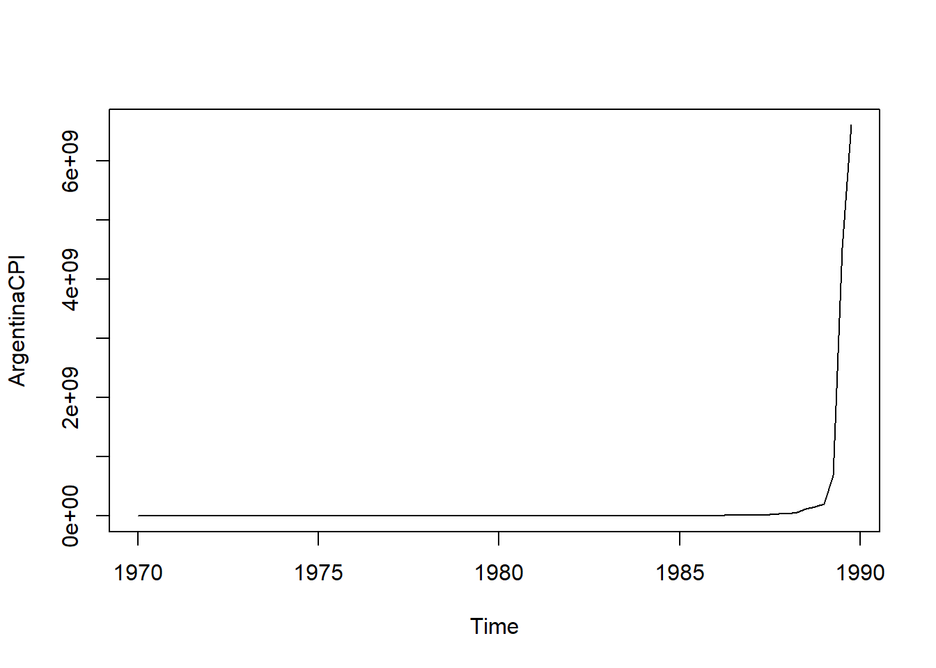

Working with ggplot() is a bit trickier: the ggplot2 package works only with data frames, and our time series object isn’t a data frame. As usual, however, if you put in enough work, and augment ggplot2 with such packages as lubridate, ggfortify, scales, and the like, time series graphs using ggplot2 do wind up looking lovely. The next bit of code transforms the CPI data into a dataframe, calculates an inflation rate, and uses some features from lubridate and scales to make a decent graph.

tempcpi <- data.frame(CPI = as.matrix(ArgentinaCPI), 
                      date = as.Date(time(ArgentinaCPI)))
tempcpi <- tempcpi %>% 
  mutate(inflation = (CPI - lag(CPI, n = 4))/lag(CPI,n = 4))
tempcpi %>% 
  ggplot(aes(x = date, y = inflation)) +
  geom_line(color = "#00573C",
            size = 1.2) +
  theme_minimal() +
  scale_y_continuous(labels = scales::label_percent(big.mark = ","),
                     expand = c(0,0)) +
  scale_x_date(expand = c(0,0),
               labels = date_format("%Y")) +
  labs(title = "Argentinian Hyperinflation",
       subtitle = "Inflation from 1970-1990",
       x = "Year",
       y = "Annualized Inflation Rate")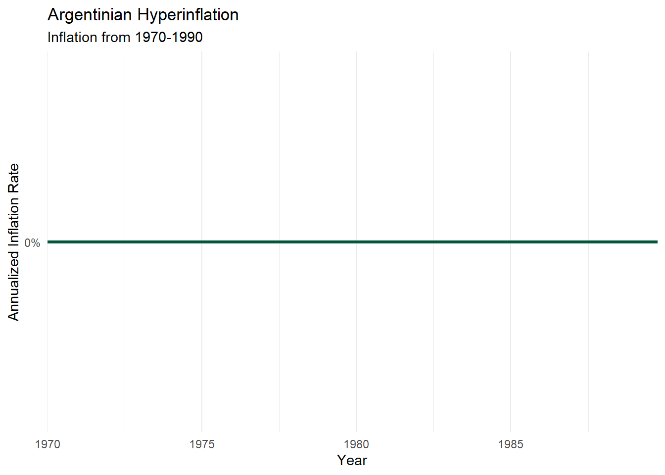

Holy cow that’s a lot of inflation!

Another method of putting time series data into ggplot2 is found in the forecast package, which we will make use of a bit later in this chapter.

Let’s prepare a different data set for time series analysis, one with multiple variables, to see what tha looks like. Above, we loaded in a dataset called okun from the wooldridge package; the description of okun is pretty spartan. The help file obtained by typing ?okun merely tells us that it is “a data.frame with 47 observations on 4 variables” and that the data comes from the Economic Report of the President, 2007. From looking at the variable descriptions, it appears that we are looking at time series data that was collected annually from 1959 to 2005 and that the variables are year, gdp growth, unemployment, and first-differenced (i.e. year-over-year change in) unemployment.

Notably, if you look at the description of the data in your environment pane, R tells us that the object okun is “47 obs. of 4 variables,” so it is not reading it as time series. This means we need to use the ts() function on it. The data description tells us that the data start in 1959, and that the data is annual, so we set the frequency paramenter to 1:

okun2 <- ts(okun, start = 1959, frequency = 1)

The new object, okun2, should appear directly underneath the original object okun in the environment window. This object is identified as a time series object: the description states “Time-Series [1:47, 1:4] from 1959 to 2005: …”. The number in the brackets tell us that there are 47 observations and 4 variables. If we look at the head() of each object, we can see that they have the same data but R treates them differently because they are different types of object:

head(okun)

##   year pcrgdp unem      cunem
## 1 1959    7.1  5.5         NA
## 2 1960    2.5  5.5  0.0000000
## 3 1961    2.3  6.7  1.1999998
## 4 1962    6.1  5.5 -1.1999998
## 5 1963    4.4  5.7  0.1999998
## 6 1964    5.8  5.2 -0.5000000

head(okun2)

## Time Series:
## Start = 1959 
## End = 1964 
## Frequency = 1 
##      year pcrgdp unem      cunem
## 1959 1959    7.1  5.5         NA
## 1960 1960    2.5  5.5  0.0000000
## 1961 1961    2.3  6.7  1.1999998
## 1962 1962    6.1  5.5 -1.1999998
## 1963 1963    4.4  5.7  0.1999998
## 1964 1964    5.8  5.2 -0.5000000

We can use the plot() function on the okun2 object; because R recognizes the whole dataset as time series, we get multiple plots!

plot(okun2)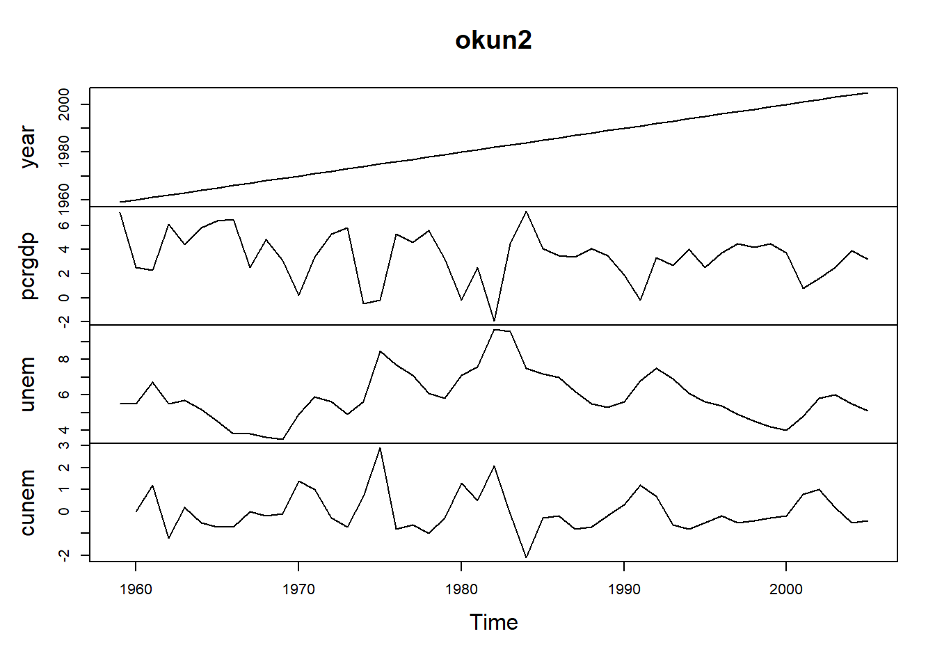

Referring to individual variables within a time series is a little bit trickier, as we can’t use the typical $ notation; trying to refer to the unemployment data as okun2$unem will result in an error. The notation that will work here is okun2[ ,"unem"], so we are essentially working with subset notation, not subobject notation.

This graph is something we would want to clean this up a bit before using; the \(year\) variable, for example, does nothing for us. We might also think about using the original version of the data, okun, in ggplot().

10.2 Autocorrelation

In Chapter 6 we discussed the issue of serial correlation or autocorrelation. Serial correlation primarily exists in time series data and it describes a data set where you can reliably predict an observation with the observation(s) that came directly before it. It’s a bit more intuitive if you think about what the word serially means; we are worried about how the data exist in a series, or in their natural order, and that consecutive data points say something about each other..

As an example, assume you live in an area with a warm temperate climate and that the average daily high temperature where you live is 75\(^\circ\)F. If the high temperature today is 95\(^\circ\)F, and I asked you to predict tomorrow’s high, what would you guess? Probably something pretty close to 95\(^\circ\)F, because it’s probably the middle of the summer if it is that hot. Similarly, if today the high temperature is 52\(^\circ\)F, your best guess for tomorrow is probably close to 52\(^\circ\)F, because it is likely the middle of February. Daily temperature is almost certainly going to have a high degree of autocorrelation, especially in a temperate climate.

Another way to think about autocorrelation is with respect to the error term of a trend line. The following code creates a (leap) year’s worth of fictitious weather data; let’s assume that this is the daily high temperatures over one year with the following characteristics:

set.seed(8675309)
rngesus <- rnorm(69, mean = 1.54, sd = 6)
bsweather1 <- runif(183, 54, 92)
bsweather1 <- sort(bsweather1, decreasing = FALSE)
bsweather1 <- bsweather1 + rngesus 
bsweather2 <- runif(183, 54, 92)
bsweather2 <- sort(bsweather2, decreasing = TRUE)
bsweather2 <- bsweather2 + rngesus 
bsweather <- c(bsweather1, bsweather2)
localweather <- ts(bsweather, start = c(2021,1), freq = 365)
summary(localweather)

##    Min. 1st Qu.  Median    Mean 3rd Qu.    Max. 
##   49.36   65.05   74.67   75.00   84.68  105.07

A time plot of this fake weather data looks like this:

plot(localweather)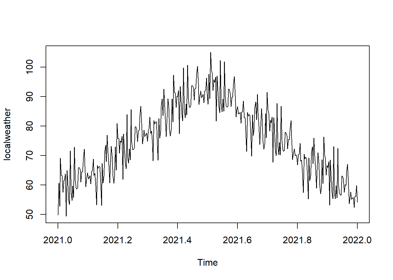

As one might suspect, average high temperatures are higher in the summer and lower in the winter, exhibiting the autocorrelation we might expect. As the mean temperature over this time period is 75\(^\circ\)F, let’s include a line at 75 in our graph:

plot(localweather)
abline(a = 75, b = 0)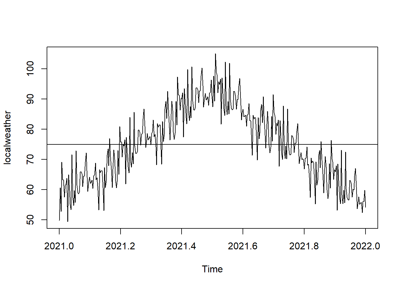

So now, if I told you that a particular observation is above the line (i.e. has a positive residual), what would you use that information to predict with respect to the next observation? You would likely predict that the next observation would also be above the line. If I told you that a particular observation is 7\(^\circ\)F below the line, your prediction should be that tthe next observation will also be 7\(^\circ\)F below the line.

This is the basic idea that autocorrelation is getting at, that residuals are serially correlated. Recall from Chapter 6, however, that we don’t want our data to have serial correlation in order to run regressions with it!

Before we get there, howeber, we can look at a couple of more formal methods to examine whether or not our data has serial correlation. We can start with an autocorrelation plot, which is generated with the acf() function.

An autocorrelation plot shows the average amount of correlation between each observation and the nth lag of that observation. Lag refers to how many observations back to look, so lag = 1 looks at the previous observation, lag = 2 the one before that, and so forth. This will make sense if we take a look at the autocorrelation plot:

acf(localweather)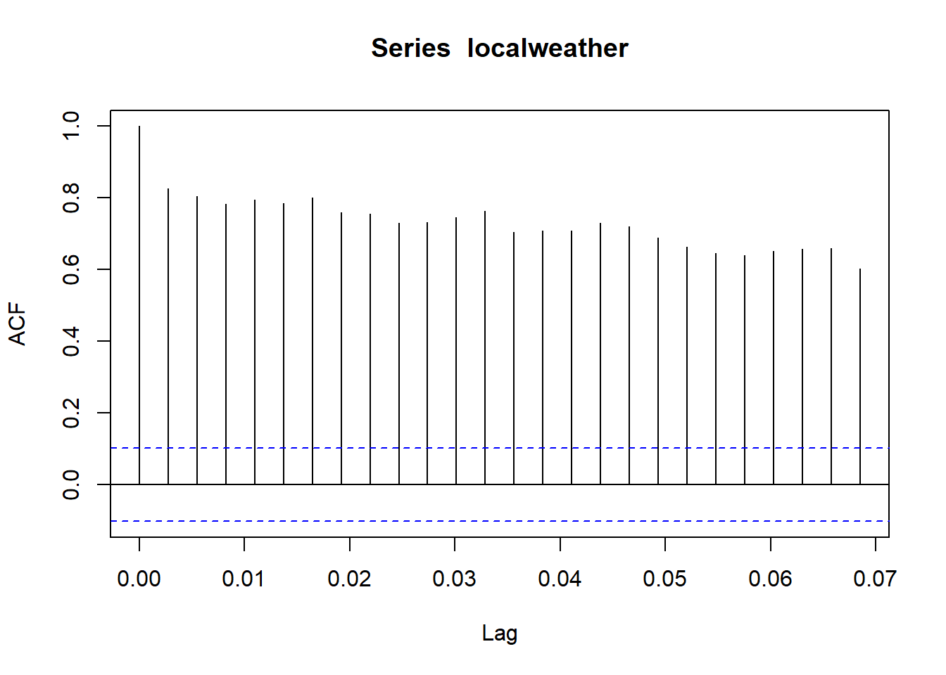

For now, let’s skip the first vertical line and focus on the second one, which looks to be around 0.83. To see what his means, let’s say we take our data and add another variable to it: yesterday’s high temperature – or, in other words, the first lag. We can explicitly do this with the Lag() function from the Hmisc package, and combine the two variables into the same dataset:

localweather1 <- Hmisc::Lag(localweather,1)
tempdat = data.frame(localweather, localweather1)

Let’s take a look at the first few rows of our tempdat object:

head(tempdat)

##   localweather localweather1
## 1     49.73926            NA
## 2     60.56603      49.73926
## 3     52.76476      60.56603
## 4     69.10110      52.76476
## 5     63.37848      69.10110
## 6     63.16129      63.37848

Recall that \(localweather\) is the daily high temperature, and \(localweather1\) is the first lag of \(localweather\). In the second row, \(localweather2\) takes on the value of \(localweather\) from row one, and so on. We can add a second and third (and so on!) lag in the same way:

localweather2 <- Hmisc::Lag(localweather, 2)
localweather3 <- Hmisc::Lag(localweather, 3)
tempdat <- data.frame(tempdat, localweather2, localweather3)
head(tempdat)

##   localweather localweather1 localweather2 localweather3
## 1     49.73926            NA            NA            NA
## 2     60.56603      49.73926            NA            NA
## 3     52.76476      60.56603      49.73926            NA
## 4     69.10110      52.76476      60.56603      49.73926
## 5     63.37848      69.10110      52.76476      60.56603
## 6     63.16129      63.37848      69.10110      52.76476

We have explicitly created 3 lags now; we already had the first lag, now we have \(localweather2\), which is the value of \(localweather\) from 2 periods ago and is thus the 2nd lag, and similarly \(localweather3\) is the value of \(localweather\) from 3 time periods ago.

You might be wondering why there are \(NA\) values in the data. This is because those lags do not exist! If data point 1 is the temperature on January 1, the first lag would be the temperature on December 31, which we do not have. So R returns a value of \(NA\).

So now that we have this data, let’s calculate the correlation between \(localweather\) and its 3 lags, making use of the use="complete.obs" option in cor to ignore the \(NA\) values:

cor(tempdat, use="complete.obs")

##               localweather localweather1 localweather2 localweather3
## localweather     1.0000000     0.8332100     0.8149322     0.7993273
## localweather1    0.8332100     1.0000000     0.8330000     0.8154749
## localweather2    0.8149322     0.8330000     1.0000000     0.8324445
## localweather3    0.7993273     0.8154749     0.8324445     1.0000000

The first row is what is important here. We can see that the correlations between \(localweather\) and its first lag is 0.834, its second lag is 0.817, and its third lag is 0.799. These numbers are what the autocorrelation plot is graphing! The 2nd through 4th bars represent the correlations between \(localweather\) and its 1st, 2nd, and 3rd lags, respectively:

acf(localweather)

What about the first vertical line? The first vertical line is the 0th lag, which basically asks whether or not \(localweather\) is correlated with \(localweather\), so by definition it will equal 1, because the observations are perfectly correlated with themselves.

Now that we see what this graph is displaying, we can use it to identify whether or not the data has autocorrelation by comparing the heights of the bars to the blue dashed lines. The blue dashed lines indicate that the correlation is significant, so we can say pretty conclusively that this data has a high degree of autocorrelation.

Now that we can see that our data has lots of autocorrelation, it is logical to think about how this issue might be fairly recursive; after all, If \(localweather\) is correlated with \(localweather1\) and \(localweather2\), doesn’t it stand to reason that \(localweather1\) is correlated with \(localweather2\)? This sort of thinking is where partial autocorrelation comes in. A partial autocorrelation graph indicates only the correlation between the data and a given level of lag that is not explained by all the shorter lags. In other words, the partial autocorrelation with the third lag \(localweather3\) looks at how much correlation exists between the \(localweather2\) and \(localweather\) that isn’t explained away by the correlation between \(localweather\) and either \(localweather1\) or \(localweather2\).

We can plot the partial autocorrelation function (PACF) with the pacf function:

pacf(localweather)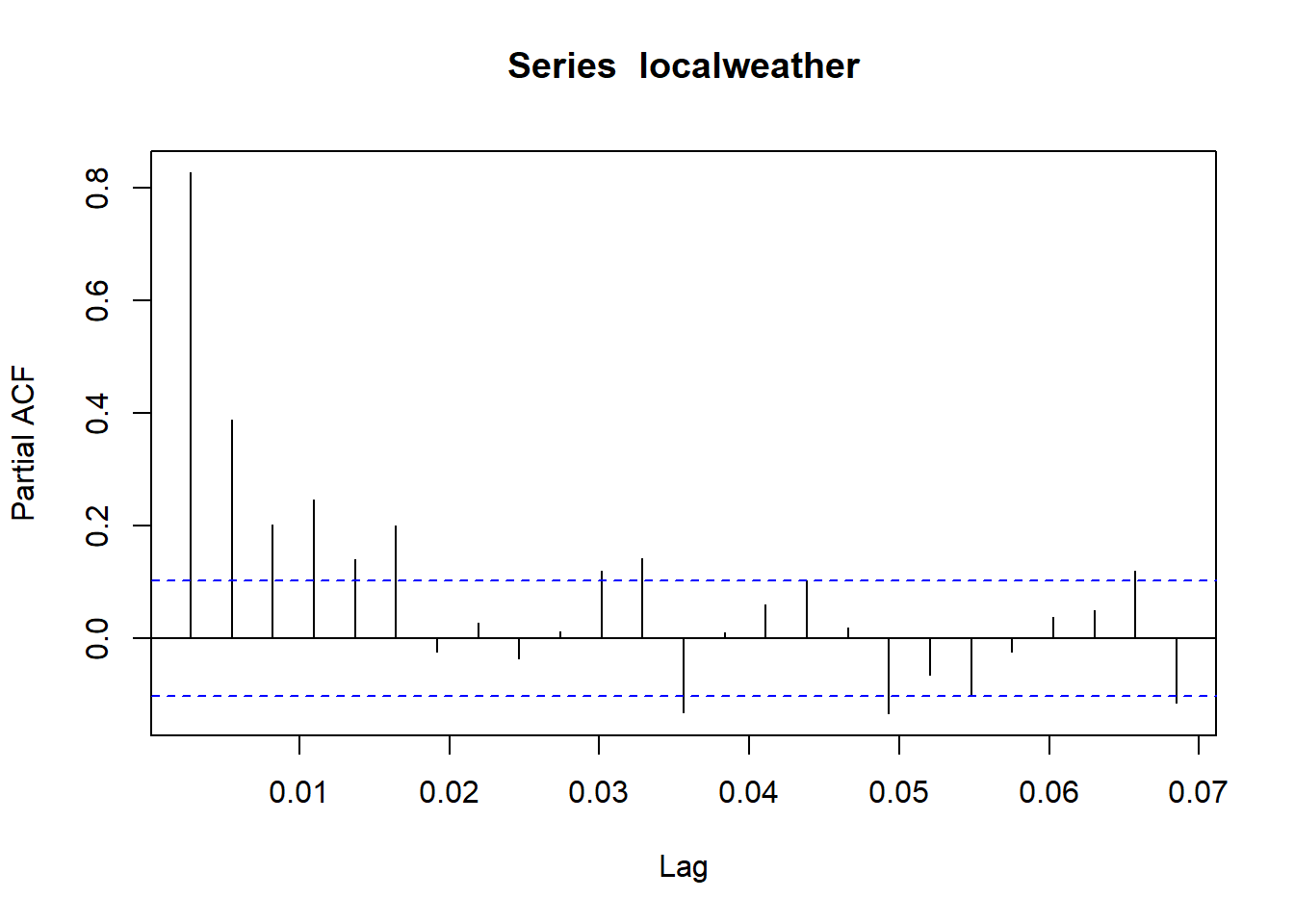

Here, we see that the PACF falls off considerably from the first to the second lag, because a huge share of the correlation between \(localweather\) and \(localweather2\) is already contained in the correlation between \(localweather\) and \(localweather1\). What does this mean? The intuition goes something like this: we know that the high correlation between \(localweather\) and \(localweather1\) tells us that, for example, if it is 85\(\circ\)F today, it is highly likely to be right around 85\(\circ\)F tomorrow. That said, let’s say it is 85\(\circ\)F in May, and while it may be the case that most days in May are 85\(\circ\)F, sometimes the day before was either unseasonably warm (say 98\(\circ\)F) or unseasonably cold (say 69\(\circ\)F). In these cases, looking at the first lag is likely to be not as good an idea as the 2nd lag, which probabilistically is likely to be closer to the May average temperature of 85\(\circ\)F than yesterdays outlier temperature of 98\(\circ\)F or 69\(\circ\)F.

10.3 Autoregression, Moving Averages, and Trends (oh my!)

When analyzing time series data, we are often looking to see if the data has any trends in either mean or variance over time. Trends can be deterministic, stochastic, or a combination of the two. We will start by looking at a little bit of the math behind these concepts.

10.3.1 Deterministic Series

A time series is deterministic if the overall function looks something like this:

\[ y_t= \omega + \gamma t + \epsilon_t \]

In this function, \(\omega\) indicates the value of the function at \(t=0\), and \(\gamma\) shows how much that \(y\) grows (or shrinks!) from one time period to the next. As usual, \(\epsilon\) serves as the error term.

This next chunk of code creates a random data with a deterministic time trend. For this data, \(\omega = 4\), \(\gamma = .7\), and \(\epsilon\) is randomly generated from the standard normal distribution. They are graphed using the autoplot function, part of the ggplot2 package that works time series:

set.seed(8675309)
count <- 1:100
rando <- rnorm(100)
tempvar <- 4 + count * .7 + rando
tempvar <- ts(tempvar, start = 1, frequency = 1)
autoplot(tempvar)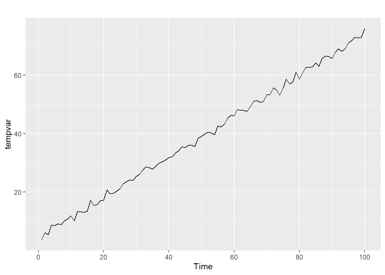

10.3.2 Autoregression

A stochastic time series, on the other hand, has a function with one or more autoregressive terms in it. We denote the autoregression within a series with the notation of AR(p), where p is the number of autoregressive lags. The math behind AR series with more than one lag can get a bit messy, so we will focus here on AR(1). Here is the generic formula for an AR(1) series; in other words, a time series with a single autoregressive lag:

\[ y_t = \phi +\rho y_{t-1} + \epsilon_t \]

Here, we have \(y_t\) as a function of \(Y_{t-1}\), so \(y_t\) will be influenced by its previous value via the parameter \(\rho\). To get a better feel for what this equation does, we generate some data to see what the impact of the parameter \(\rho\) is. We will start by looking at situations where \(0 \geq \rho >1\). In this range, \(\rho\) is a measure of how persistent the fluctuations in the data are.

Assume that at \(t=1\), \(\epsilon\) is a really big positive outlier, so \(y_1\) is a lot bigger than the expected value of \(y_1\). The impact this has on \(y_2\) is determined by \(\rho\). If \(\rho\) is zero, the extraordinarily high value of \(y_1\) doesn’t impact \(y_2\) at all; \(y_2\) is determined entirely by \(\phi\) and \(\epsilon_2\). The higher is \(\rho\), the bigger the effect that \(y_1\) will have on determining the value of \(y_2\). In short, as \(\rho\) gets close to 1, you start to see cycles in the data, because outliers in the data will persist more to the next period.

The code below creates 5 AR(1) series of 200 observations each with the arima.sim() function. The first series, \(ardata00\), uses a value of \(\rho=0\), so the \(y_{t-1}\) term drops out of the equation altogether. The resulting time series is white noise. The other four time series use values for \(\rho\) of 0.5, 0.75, 0.9, and 0.99, respectively. These time series are then graphed below, the data with the highest \(\rho\) is the series on top, and the graphs are presented in decending \(\rho\) order:

set.seed(8675309)
ardata00 <- arima.sim(list(order = c(0,0,0)), n = 200)
ardata50 <- 10 + arima.sim(list(order = c(1,0,0), ar = .5), n = 200)
ardata75 <- 20 + arima.sim(list(order = c(1,0,0), ar = .75), n = 200)
ardata90 <- 30 + arima.sim(list(order = c(1,0,0), ar = .90), n = 200)
ardata99 <- 40 + arima.sim(list(order = c(1,0,0), ar = .99), n = 200)

# Note that the addition of 10, 20, 30, and 40 are simply for spacing and allow
# the next bit of code to put them together clearly on the same graph.

autoplot(ardata00) +
  autolayer(ardata50) +
  autolayer(ardata75) +
  autolayer(ardata90) +
  autolayer(ardata99) +
  theme(axis.text.y=element_blank()) + 
  scale_y_discrete(breaks=NULL) +
  geom_hline(yintercept = 0, linetype = 2, alpha = .5) +
  geom_hline(yintercept = 10, linetype = 2, alpha = .5) +
  geom_hline(yintercept = 20, linetype = 2, alpha = .5) +
  geom_hline(yintercept = 30, linetype = 2, alpha = .5) +
  geom_hline(yintercept = 40, linetype = 2, alpha = .5) +
  ylab("") +
  theme_minimal()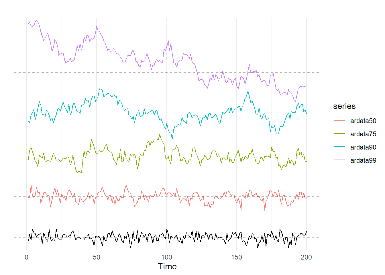

What are you supposed to see here? The white noise graph on the bottom shouldn’t look like much of anything, as by design there are no real patterns in the data. As \(\rho\) increases, we start to see the appearance of cycles in the data. For example, \(ardata90\) looks like it is increasing for the first 50 observations or so, then decreasing for the next 55 observations, followed by a slow increase over the next 70 periods, and then it crashes! The top graph of \(ardata99\) looks it has an overall downward trend in the data. None of these patterns are by design: you can check the code for yourself, none of those things were coded into the number generation process. In fact, you can take the code above and change the set.seed() option to any other number (or just comment out the command with #) and generate a new set of 5 time series for every seed you put in; you will see that the \(\rho=0\) line generally looks the similar every time, but as \(\rho\) increases, you start to see cycles and trends in the data. This is simply the result of an AR(1) process with a value of \(\rho\) very close to one!

We can also look at what happens when \(\rho\) takes on values in the range of \(-1 >\rho \geq 0\). Similar to the above case, the closer \(\rho\) gets to -1, the more previous values will persist in the data from one period to the next. However, because \(\rho\) is negative, it forces the sign to flip so you wind up with a series with a lot of oscillation. The following code creates time series of 50 observations with values of rho equal to -0.5, -0.75, -0.9, and -0.99. These results are then graphed using the autoplot function:

set.seed(12345)
ardatan00 <- ardata00[1:50]
ardatan00 <- ts(ardatan00)
ardatan50 <- 10 + arima.sim(list(order = c(1,0,0), ar = -.5), n = 50)
ardatan75 <- 20 + arima.sim(list(order = c(1,0,0), ar = -.75), n = 50)
ardatan90 <- 30 + arima.sim(list(order = c(1,0,0), ar = -.90), n = 50)
ardatan99 <- 40 + arima.sim(list(order = c(1,0,0), ar = -.99), n = 50)

autoplot(ardatan00) +
  autolayer(ardatan50) +
  autolayer(ardatan75) +
  autolayer(ardatan90) +
  autolayer(ardatan99) +
  theme(axis.text.y=element_blank()) + 
  scale_y_discrete(breaks=NULL) +
  geom_hline(yintercept = 0, linetype = 2, alpha = .5) +
  geom_hline(yintercept = 10, linetype = 2, alpha = .5) +
  geom_hline(yintercept = 20, linetype = 2, alpha = .5) +
  geom_hline(yintercept = 30, linetype = 2, alpha = .5) +
  geom_hline(yintercept = 40, linetype = 2, alpha = .5) +
  ylab("") +
  theme_minimal()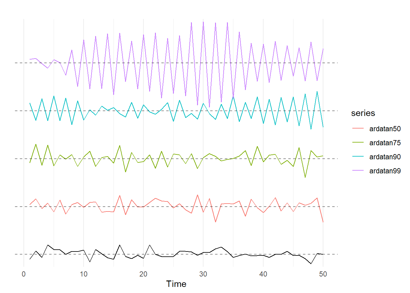

Again, the bottom line is white noise. As \(\rho\) gets closer to -1, the data starts to oscillate (switch back and forth between positive and negative) and increase in variance (in other words, the amplitude of the oscillation tends to increase). Again, to get a feel for how \(\rho\) affects the AR(1) series, copy the code from above and change the seed to see different time series generated with different values of \(\rho\).

So far we have looked at how an AR(1) process behaves if \(-1 <\rho < 1\). If an AR(1) process has \(-1 <\rho < 1\), it is said to be stationary, which means that the time series has a constant mean and variance. To see the intuition of this, recall the AR(1) equation: \(y_t = \phi +\rho y_{t-1} + \epsilon_t\). In this equation, if \(-1 <\rho < 1\), because the expected value of \(\epsilon_t\) is \(E[\epsilon_t]=0\), the tendency is for \(y_t\) to be closer to \(\phi\) than is \(y_{t-1}\).

Generally speaking, when we are doing time series econometrics we really want our data to be stationary.

However, it isn’t always, so let’s turn to nonstationary data. If \(|\rho|=1\), a time series is said to have a unit root and is often called a random walk. A random walk is not stationary because the variance of the data increases over time. Recall that the equation for an AR(1) process is \(y_t = \phi +\rho y_{t-1} + \epsilon_t\). For simplicity, assume that \(\phi=0\). If \(\rho=1\), this equation simplifies to \(y_t = y_{t-1} + \epsilon_t\). Unlike the situation above when \(|\rho|<1\), there is nothing that is “pushing” the time series back to 0. If \(\epsilon_3\) happens to be a big number, the series becomes permanently higher, because the best predictor of \(y_4\) is \(y_3\).

The code below creates and graphs 4 random walks with mean 0 and \(\sigma=1\); again, the bottom line is a random walk for comparsion. As with the above sets of graphs, I’d suggest copying the code into R and changing the number in the set.seed() command to see a bunch of examples of what random walks look like.

set.seed(8675309)
ardata00 <- arima.sim(list(order = c(0,0,0)), n = 200)
rwalk1 <- 20 + cumsum(rnorm(200,0,1))
rwalk1 <- ts(rwalk1)
rwalk2 <- 40 + cumsum(rnorm(200,0,1))
rwalk2 <- ts(rwalk2)
rwalk3 <- 60 + cumsum(rnorm(200,0,1))
rwalk3 <- ts(rwalk3)
rwalk4 <- 80 + cumsum(rnorm(200,0,1))
rwalk4 <- ts(rwalk4)

autoplot(ardata00) +
  autolayer(rwalk1) +
  autolayer(rwalk2) +
  autolayer(rwalk3) +
  autolayer(rwalk4) +
  theme(axis.text.y=element_blank()) + 
  scale_y_discrete(breaks=NULL) +
  geom_hline(yintercept = 0, linetype = 2, alpha = .5) +
  geom_hline(yintercept = 20, linetype = 2, alpha = .5) +
  geom_hline(yintercept = 40, linetype = 2, alpha = .5) +
  geom_hline(yintercept = 60, linetype = 2, alpha = .5) +
  geom_hline(yintercept = 80, linetype = 2, alpha = .5) +
  ylab("") +
  theme_minimal()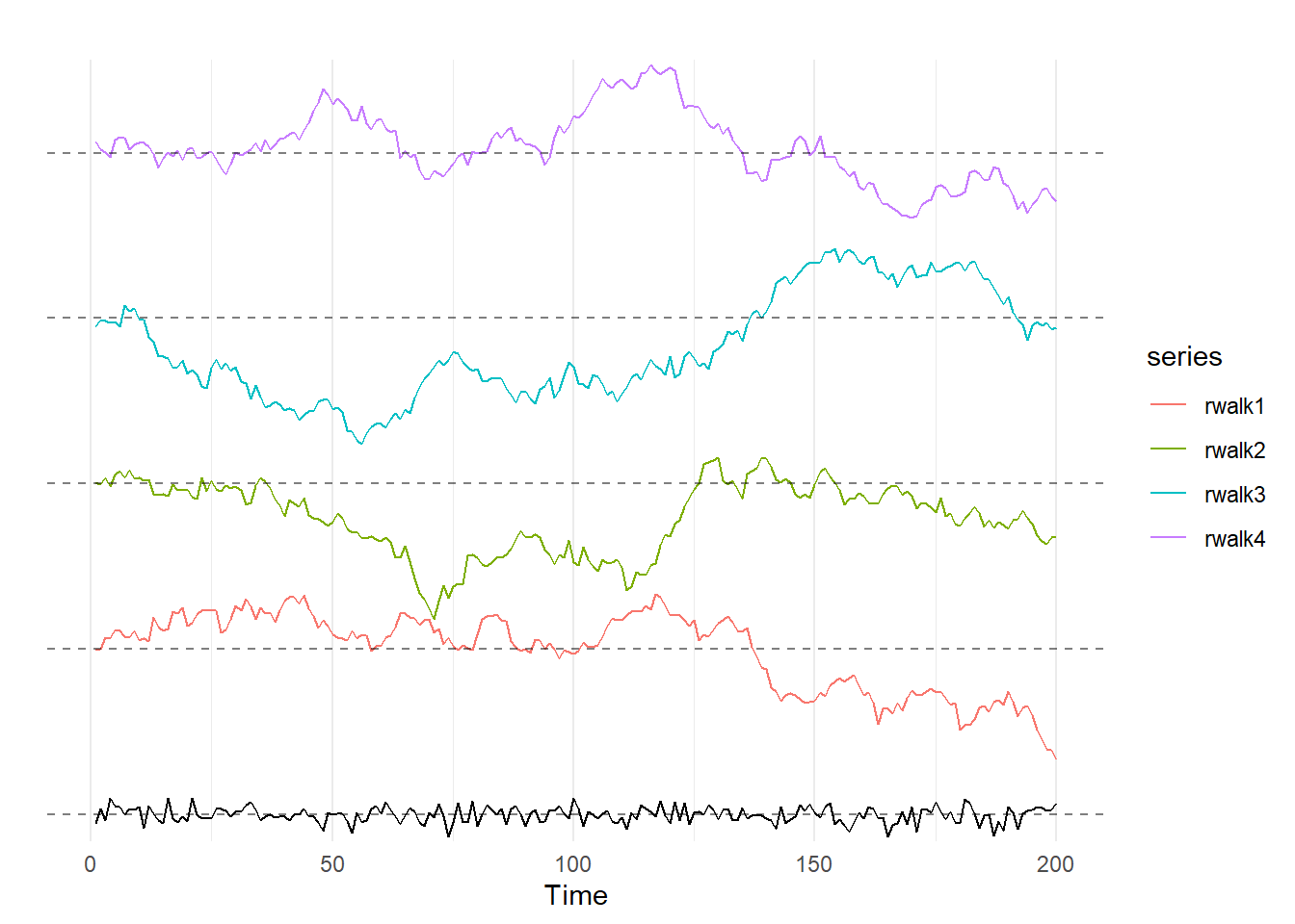

Generally speaking, when trying to model a time series with a unit root we need to first-difference our data; we will discuss first-differencing below when we get to time trends. Finally, if \(|\rho| \geq 1\), the time series is termed to be explosive. If a time series is explosive, it generally requires more extensive transformation, like log transformation.

10.3.3 Moving Average Series

A moving average series has a lot of similarities with an autoregressive series. Whereas an AR(p) series included \(p\) lags of the variable y, a moving average series MA(q) includes \(q\) lags of the error term, \(\epsilon\)!

A basic MA(1) model takes the following form:

\[ y_t = \phi + \epsilon_t + \theta \epsilon_{t-1} \]

We can see what happens in our MA models as we allow \(\theta\) to vary from 0 to 0.99:

set.seed(8675309)
madata00 <- arima.sim(list(order = c(0,0,0)), n = 200)
madata50 <- 10 + arima.sim(list(order = c(0,0,1), ma = .5), n = 200)
madata75 <- 20 + arima.sim(list(order = c(0,0,1), ma = .75), n = 200)
madata90 <- 30 + arima.sim(list(order = c(0,0,1), ma = .90), n = 200)
madata99 <- 40 + arima.sim(list(order = c(0,0,1), ma = .99), n = 200)

# Note that the addition of 10, 20, 30, and 40 are simply for spacing and allow
# the next bit of code to put them together clearly on the same graph.

autoplot(madata00) +
  autolayer(madata50) +
  autolayer(madata75) +
  autolayer(madata90) +
  autolayer(madata99) +
  theme(axis.text.y=element_blank()) + 
  scale_y_discrete(breaks=NULL) +
  geom_hline(yintercept = 0, linetype = 2, alpha = .5) +
  geom_hline(yintercept = 10, linetype = 2, alpha = .5) +
  geom_hline(yintercept = 20, linetype = 2, alpha = .5) +
  geom_hline(yintercept = 30, linetype = 2, alpha = .5) +
  geom_hline(yintercept = 40, linetype = 2, alpha = .5) +
  ylab("") +
  theme_minimal()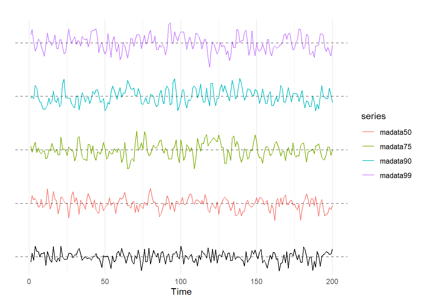

Unlike in the AR models, they don’t look all that different. We see a bit more cyclicality at higher values of \(\theta\), but nothing like what we saw with an AR model with \(\rho\) cranked up. This is because the MA(1) model only carries over the error term from one time period to the next, as opposed to \(y\).

Assume that in time period 1, the error term, \(\epsilon_1\), is a large positive number. In an AR(1) model with \(\rho=0.99\), that large error term would make \(y_1\) large. Because \(y_1\) is large, this means \(y_2\) will probably be pretty big too because the equation for \(y_2\) includes \(\rho y_1\). And since \(y_2\) is large, so too would we expect \(y_3\), \(y_4\), and so forth, because with \(\rho=0.99\) it may take a long time for the abnormally \(\epsilon_1\) to work its way out.

By contrast, if the error term in period 1 is a large positive number in an MA(1) model with \(\theta = .99\), the fact that \(y_1\) is large does not impact the value of \(y_2\). However, \(y_2\) will be impacted by \(\epsilon_1\), and since \(\epsilon_1\) is large, we expect \(y_2\) to be large as well. But what about \(y_3\)? If the MA process only has one lag, then \(\epsilon_1\) won’t show up in the equation for \(y_3\), \(\epsilon_2\) will. What this all means is that crazy big (or small) outliner an MA(\(q\)) model only persists for \(q\) periods after it happens, so the larger is \(q\), the longer shocks will persist for and thus generate cycles.

To see this, consider the moving averages series below; from the bottom, these series are a random walk, an MA(1), MA(3), MA(6), and MA(9).

set.seed(8675309)
madata00 <- arima.sim(list(order = c(0,0,0)), n = 200)
madata1 <- 10 + arima.sim(list(ma = .9), n = 200)
madata3 <- 20 + arima.sim(list(ma = c(.9,.9,.9)), n = 200)
madata6 <- 30 + arima.sim(list(ma = c(.9,.9,.9,.9,.9,.9)), n = 200)
madata9 <- 40 + arima.sim(list(ma = c(.9,.9,.9,.9,.9,.9,.9,.9,.9)), n = 200)

# Note that the addition of 10, 20, 30, and 40 are simply for spacing and allow
# the next bit of code to put them together clearly on the same graph.

autoplot(madata00) +
  autolayer(madata1) +
  autolayer(madata3) +
  autolayer(madata6) +
  autolayer(madata9) +
  theme(axis.text.y=element_blank()) + 
  scale_y_discrete(breaks=NULL) +
  geom_hline(yintercept = 0, linetype = 2, alpha = .5) +
  geom_hline(yintercept = 10, linetype = 2, alpha = .5) +
  geom_hline(yintercept = 20, linetype = 2, alpha = .5) +
  geom_hline(yintercept = 30, linetype = 2, alpha = .5) +
  geom_hline(yintercept = 40, linetype = 2, alpha = .5) +
  ylab("") +
  theme_minimal()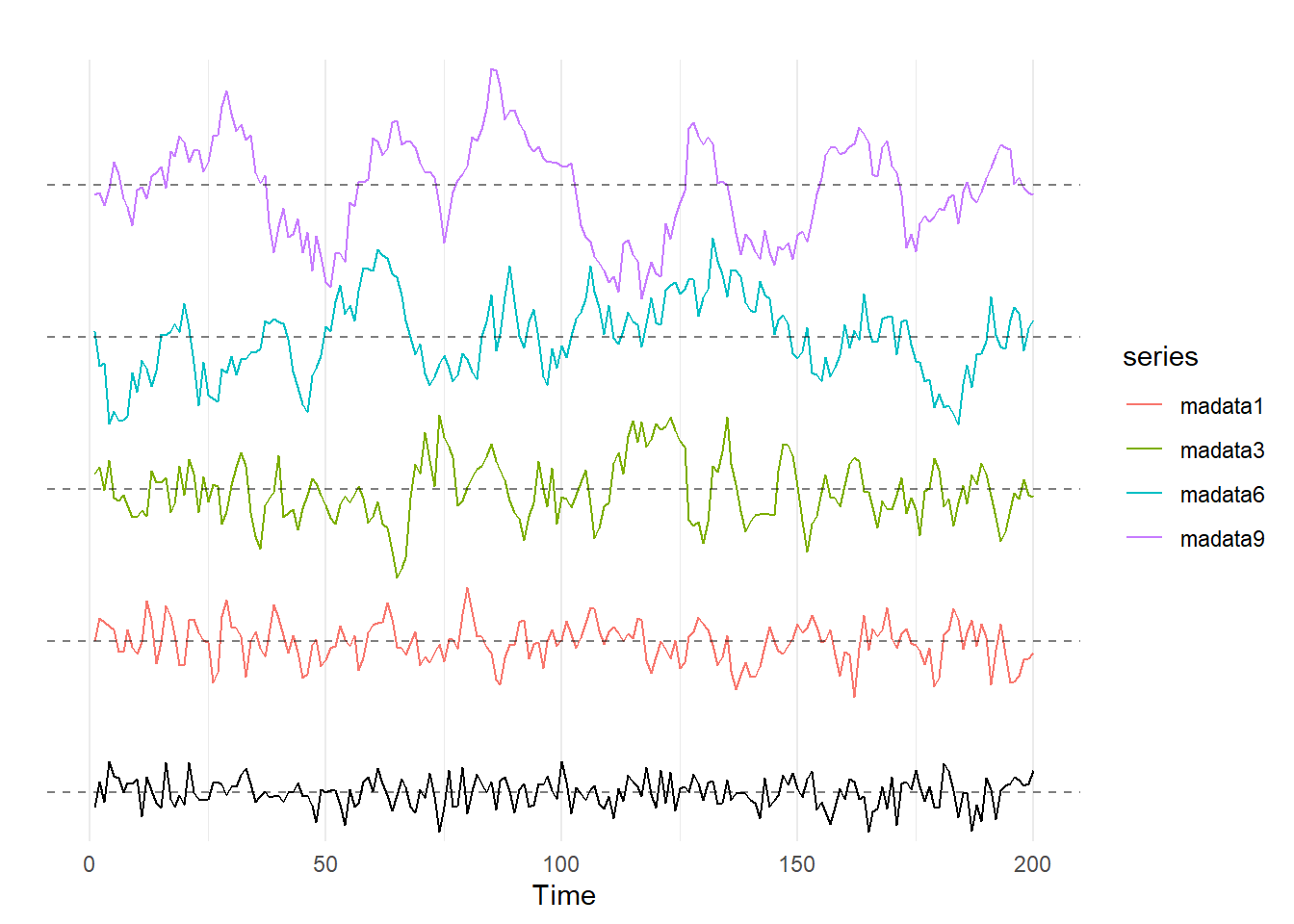

As we see here, the larger the value of \(q\) in our MA(\(q\)) series, the more likely are cycles to exist in the data.

10.3.4 ARMA Processes

An ARMA(p,q) process is a time series with both \(p\) autoregressive terms and \(q\) moving average terms. As you might suspect, an ARMA process combines the intuition of the AR and MA concepts discussed above. Below, I show some examples of ARMA(1,1) processes with both positive and negative values of \(\theta\) and \(\rho\):

set.seed(8675309)
ardata00 <- arima.sim(list(order = c(0,0,0)), n = 200)
armadata1 <- 10 + arima.sim(list(order = c(1,0,1), ar = .8, ma = .8), n = 200)
armadata2 <- 20 + arima.sim(list(order = c(1,0,1), ar = -.8, ma = -.8), n = 200)
armadata3 <- 30 + arima.sim(list(order = c(1,0,1), ar = -.8, ma = .8), n = 200)
armadata4 <- 40 + arima.sim(list(order = c(1,0,1), ar = .8, ma = -.8), n = 200)

# Note that the addition of 10, 20, 30, and 40 are simply for spacing and allow
# the next bit of code to put them together clearly on the same graph.

autoplot(ardata00) +
  autolayer(armadata1) +
  autolayer(armadata2) +
  autolayer(armadata3) +
  autolayer(armadata4) +
  theme(axis.text.y=element_blank()) + 
  scale_y_discrete(breaks=NULL) +
  geom_hline(yintercept = 0, linetype = 2, alpha = .5) +
  geom_hline(yintercept = 10, linetype = 2, alpha = .5) +
  geom_hline(yintercept = 20, linetype = 2, alpha = .5) +
  geom_hline(yintercept = 30, linetype = 2, alpha = .5) +
  geom_hline(yintercept = 40, linetype = 2, alpha = .5) +
  ylab("") +
  theme_minimal()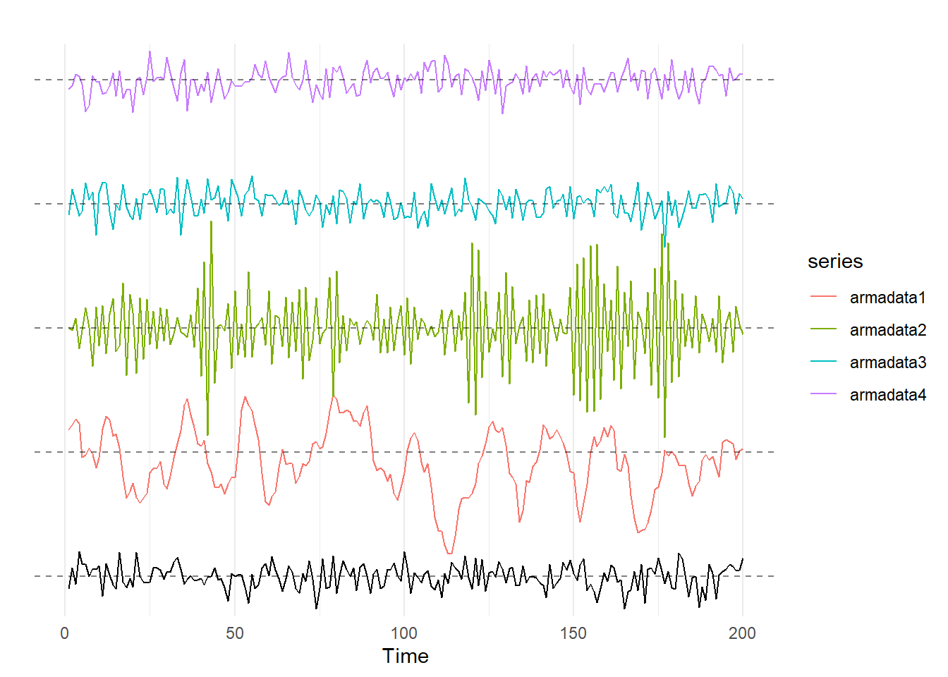

These graphs are fairly interesting. The red curve has \(\theta=0.8\) and \(\rho=0.8\), and the graph winds up looking like it has a really high value of \(\rho\) or is an MA(\(q\)) with \(\theta>0\) and a huge \(q\). Similarly, the green curve has \(\theta=-0.8\) and \(\rho=-0.8\), and that graph looks like it has \(\rho\) close to negative 1.

Even more interesting are the purple and blue lines; these have \(\theta=0.8\) and \(\rho=-0.8\) and \(\theta==0.8\) and \(\rho=0.8\), respectively, and they look a whole lot like the black white noise graph at the bottom! The lesson here is that you can’t always just look at a time series and pick out the AR and MA processes via visual inspection.

10.3.5 Trends

Suppose we have a time series that looks like this:

set.seed(8675309)
arimadata1 <- arima.sim(list(order = c(1,0,0), ar = c(.9)), n = 200)
trend <- 1:200
arimadata1 <- arimadata1 + .08 * trend


autoplot(arimadata1) +
  theme(axis.text.y=element_blank()) + 
  geom_smooth(method = lm, linetype = "dashed", color = "black", se = FALSE) +
  scale_y_discrete(breaks=NULL) +
  ylab("") +
  theme_minimal()

## `geom_smooth()` using formula 'y ~ x'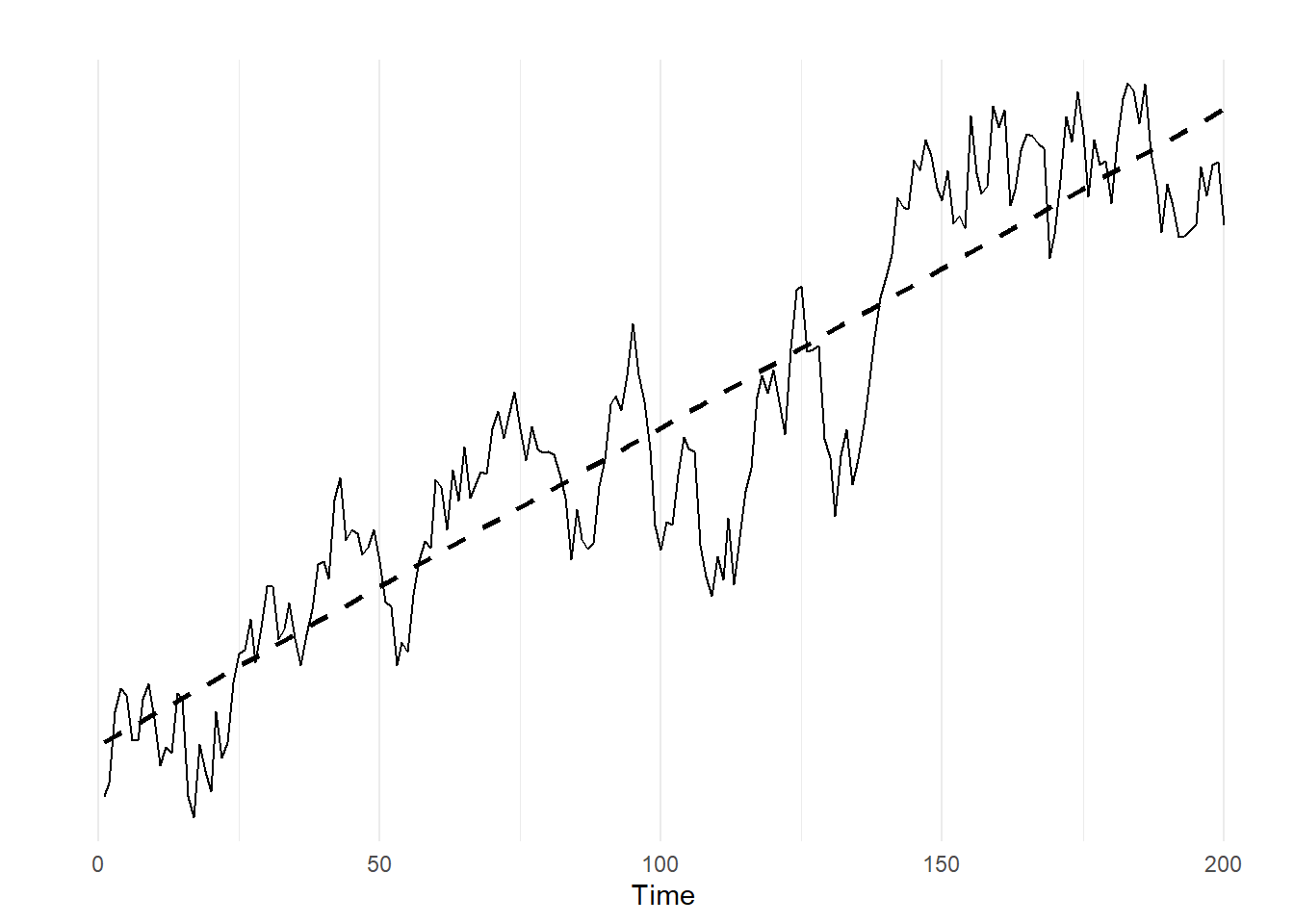

This is an AR(1) series with \(\rho=.9\) that I have added a time trend to. In order to be able to use ARMA-type modeling on this data, we need to find a way to remove the time trend, because right now the data is non-stationary.

There are two primary ways to remove the time trend: detrending and differencing

To detrend a time series variable, you:

1. Create a variable that is a time trend (e.g. a sequence of numbers from 1 to \(n\), where \(n\) is your number of observations),

2. Estimate a simple OLS regression of your time series with the trend on the time trend variable, and

3. Use the residuals as your de-trended data.

With the arimadata data from the previous bit of code, this can be accomplished by:

arimadata2 <- data.frame(arimadata1) # Convert time series to data frame
arimadata2 <- arimadata2 %>%  
  mutate(time = row_number()) # Use tidyverse to create time trend variable
detrendreg <- lm(arimadata1 ~ time, data = arimadata2) # Estimate regression
arimadata2$resids <- detrendreg$residuals # grab residuals

Now, we can look at graphs of the residuals and the original data to compare:

graph1 <- ggplot(arimadata2, aes(x = time, y = arimadata1)) +
  geom_line() +
  geom_smooth(method = lm, se = FALSE)

graph2 <- ggplot(arimadata2, aes(x = time, y = resids)) +
  geom_line() +
  geom_smooth(method = lm, se = FALSE)

cowplot::plot_grid(graph1, graph2, ncol = 1, align = "v")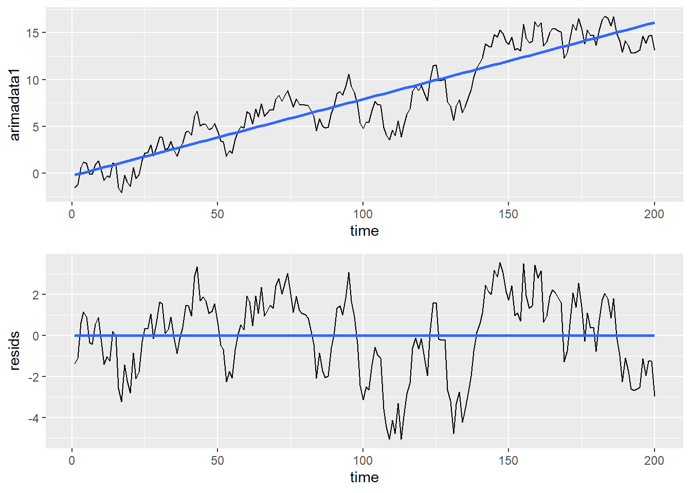

Because the residuals from the detrending regression represent the distance the time series is from the time trend in the top panel, the bottom graph retains same variation pattern as the top.

The other primary way of removing a time trend is to difference the data; if a process can be made stationary via differencing it is referred to as an Integrated time series. The most common type of differencing is called first-differencing; this means you take your data series and subtract each observation from the observation immediately before it. The easiest way to first difference a variable is with the collapse::D() function (because Base R has a D() function as well, can’t just load the collapse library and run it with D()). This next code chunk creates a first difference variable and displays the first few lines of data:

arimadata2$diff <- collapse::D(arimadata2$arimadata1)
head(arimadata2)

##   arimadata1 time     resids       diff
## 1 -1.5343131    1 -1.3652896         NA
## 2 -1.1909146    2 -1.1034840  0.3433984
## 3  0.6211683    3  0.6270061  1.8120829
## 4  1.2271355    4  1.1513805  0.6059672
## 5  1.0610602    5  0.9037125 -0.1660753
## 6 -0.1005131    6 -0.3394537 -1.1615733

The first value for \(diff\) is \(NA\). This is because you can’t take a first difference of the first data point, since there is no data point to subtract from. After that, we can see that the second data point is 0.3433984. This is the difference between the 2nd and 1st values of \(arimadata1\), or -1.1909146 - -1.5343131.

Let’s look at this new data series and compare it with both the original data and the detrended data:

graph1 <- ggplot(arimadata2, aes(x = time, y = arimadata1)) +
  geom_line() +
  geom_smooth(method = lm, se = FALSE)

graph2 <- ggplot(arimadata2, aes(x = time, y = resids)) +
  geom_line() +
  geom_smooth(method = lm, se = FALSE)

graph3 <- ggplot(arimadata2, aes(x = time, y = diff)) +
  geom_line() +
  geom_smooth(method = lm, se = FALSE)


cowplot::plot_grid(graph1, graph2, graph3, ncol = 1, align = "v")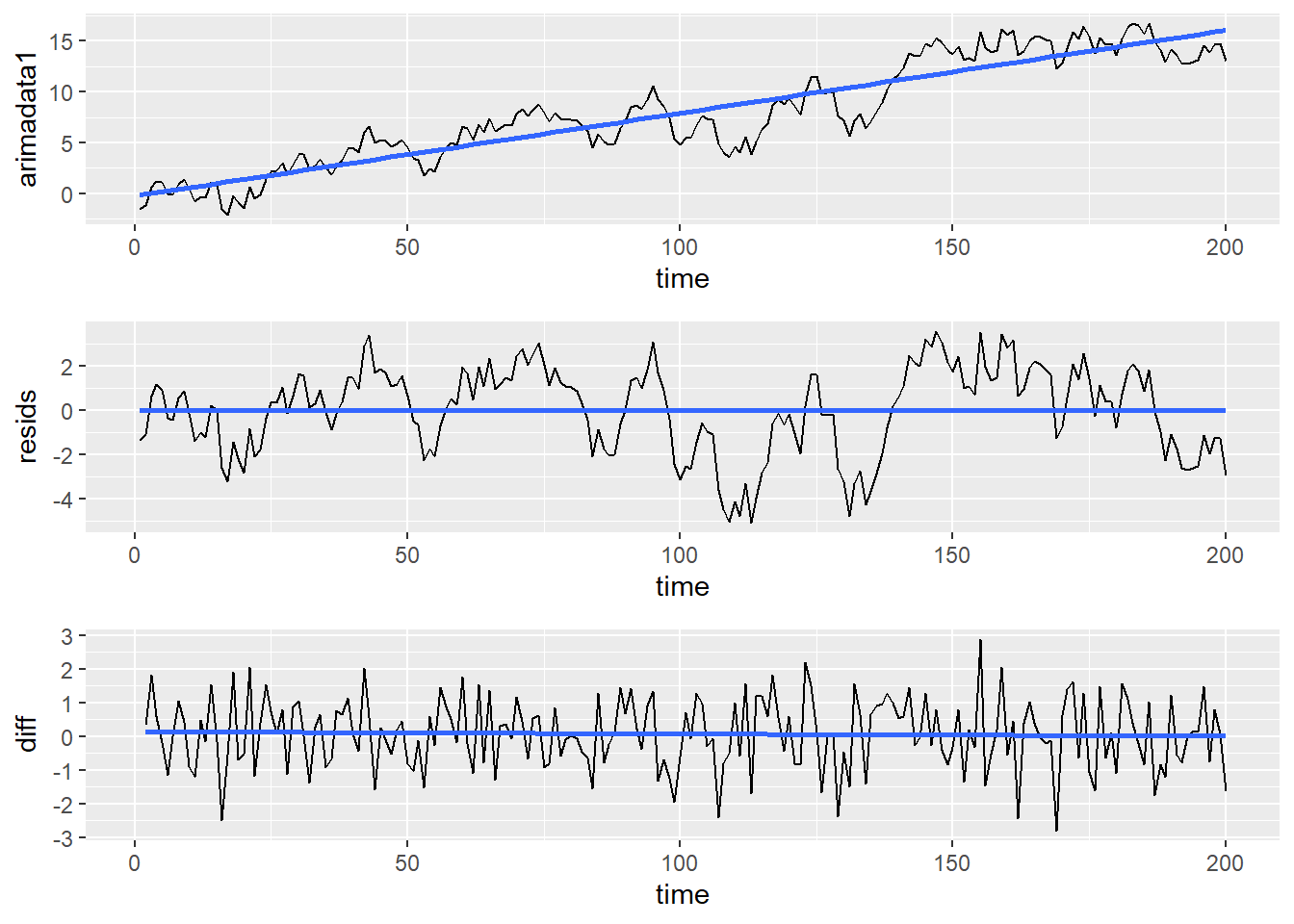

Unlike the residual data, it does not have the same variation pattern as the the original data. However, it does appear to be stationary, which is what we are going for when we are removing the trend from data.

10.4 The Dickey-Fuller Test

A common test to see if data is stationary is the Augmented Dickey-Fuller test. You can find the Augmented Dickey-Fuller test in the tseries package. The test itself is easy to run; once you have loaded tseries into memory, the function is adf.test(). The null hypothesis of the Dickey-Fuller test is that the data is explosive; rejecting the null, therefore, is evidence that the data is stationary.

Let’s look at 4 data series: \(unem\) and \(pcrgdp\) from the okun data, \(NYSESW\) (\(NYSESW\) is a zoo object, which is like a ts object but more functional), and \(BondYield\). We can start by visually inspecting these four series graphically:

autoplot(okun2[,"unem"])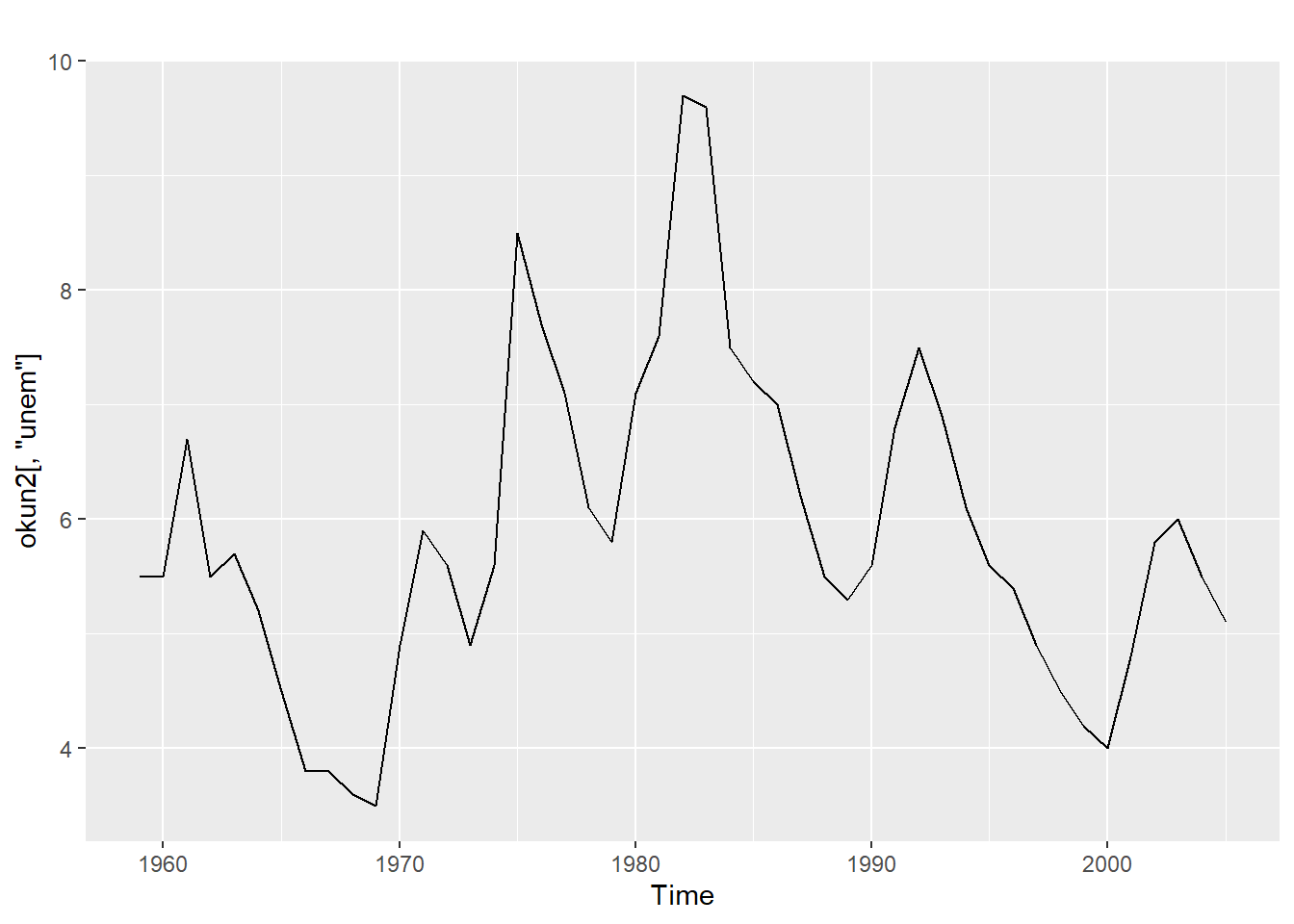

autoplot(okun2[,"pcrgdp"])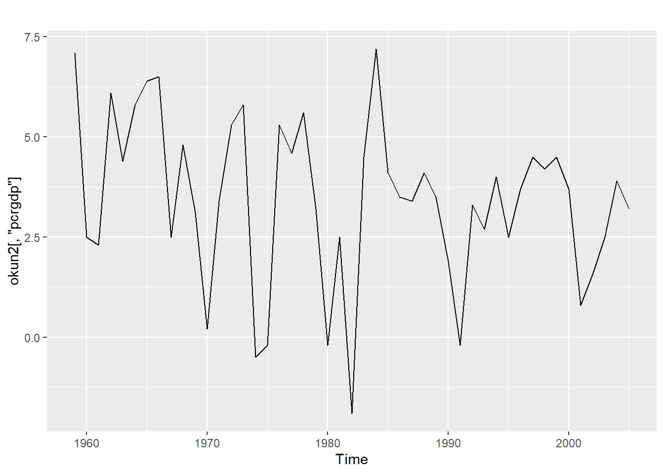

autoplot(BondYield)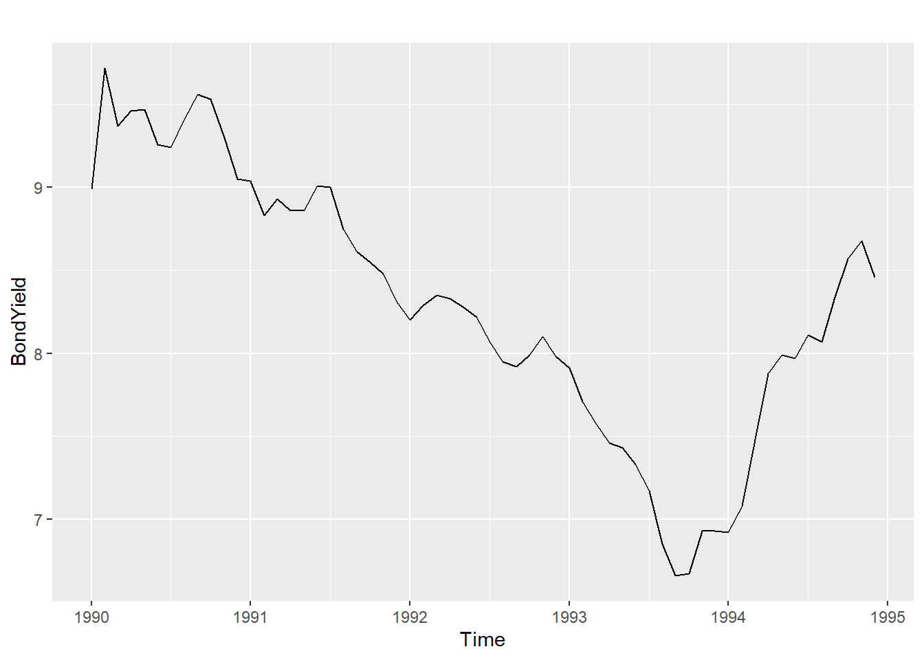

autoplot(NYSESW)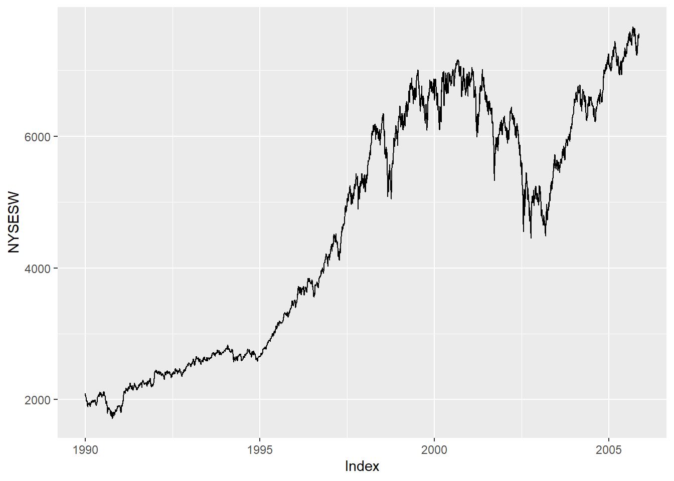

At first glance we may suspect that the first two series are stationary while the next two are not, but as mentioned above, looks can be deceiving when it comes to visually identifying time series.

Let’s subject each of these time series to the Augmented Dickey-Fuller test. Recall, the null hypothesis is that the data is explosive, so rejecting the null implies that he data is stationary.

adf.test(okun2[,"unem"])

## 
##  Augmented Dickey-Fuller Test
## 
## data:  okun2[, "unem"]
## Dickey-Fuller = -1.9331, Lag order = 3, p-value = 0.6007
## alternative hypothesis: stationary

adf.test(okun2[,"pcrgdp"])

## Warning in adf.test(okun2[, "pcrgdp"]): p-value smaller than printed p-value

## 
##  Augmented Dickey-Fuller Test
## 
## data:  okun2[, "pcrgdp"]
## Dickey-Fuller = -4.2765, Lag order = 3, p-value = 0.01
## alternative hypothesis: stationary

adf.test(BondYield)

## 
##  Augmented Dickey-Fuller Test
## 
## data:  BondYield
## Dickey-Fuller = -0.71969, Lag order = 3, p-value = 0.9635
## alternative hypothesis: stationary

adf.test(NYSESW)

## 
##  Augmented Dickey-Fuller Test
## 
## data:  NYSESW
## Dickey-Fuller = -1.8683, Lag order = 15, p-value = 0.6341
## alternative hypothesis: stationary

Looking at the results, we would conclude that only the \(pcrgdp\) series from the okun2 data is stationary.

10.5 Modeling ARIMA

When analyzing a time series, we typically want to identify all of the features discussed above in that series; the most common way of doing so is with an ARIMA model. Arima combines Autoregression (AR), Integration (I), and Moving Average (MA) processes into one model. So how do we go about identifying these characteristics of our time series?

Luckily for us, the forecast package has a very useful function called auto.arima() that does most of the hard work. This function will estimate ARIMA models of our data using multiple combinations of AR(\(p\)), MA(\(q\)), and I(\(d\)), and choose the one with the best AIC or BIC.

Let’s see this in action with the \(pcrgdp\) variable from the okun2 data:

auto.arima(okun2[,"pcrgdp"])

## Series: okun2[, "pcrgdp"] 
## ARIMA(0,0,1) with non-zero mean 
## 
## Coefficients:
##          ma1    mean
##       0.3305  3.4634
## s.e.  0.1667  0.3823
## 
## sigma^2 = 4.094:  log likelihood = -98.85
## AIC=203.69   AICc=204.25   BIC=209.24

The numbers in parenthesis following ARIMA are what tell us the ARIMA parameters. This is read as ARIMA(p, d, q), so we can say that the \(pcrgdp\) model is best fit with AR(0), I(0), and MA(1). We can also see the estimated value of \(\theta\) for our MA term: \(\theta_1=0.33\).

In similar fashion, we can use auto.arima() on the \(unem\) and \(NYSESW\) variables to identify the best fitting ARIMAs:

auto.arima(okun2[,"unem"])

## Series: okun2[, "unem"] 
## ARIMA(1,0,1) with non-zero mean 
## 
## Coefficients:
##          ar1     ma1    mean
##       0.6533  0.4142  5.8486
## s.e.  0.1307  0.1757  0.4524
## 
## sigma^2 = 0.6724:  log likelihood = -56.42
## AIC=120.85   AICc=121.8   BIC=128.25

auto.arima(NYSESW)

## Series: NYSESW 
## ARIMA(0,1,0) 
## 
## sigma^2 = 1845:  log likelihood = -21207.67
## AIC=42417.35   AICc=42417.35   BIC=42424.01

The ARIMA that best fits the \(unem\) variable is an ARMA with AR(1) with \(\rho=0.65\) and MA(1) with \(\theta=0.41\).

The \(NYSESW\) is best modeled without any AR or MA terms; the best model here only requires first differencing the data!

10.6 Forecasting

The basic idea of forecasting is to use the time trend estimated from an ARIMA model to predict the future vaules of our time series data. By its very nature, forecasting tends to be extrapolative in nature, as you are assume that the patterns that existed in the past will continue to exist into the future. There is, of course, no such guarantee in the real world!

This is why, when we forecast, we have “tighter” predictions of the near future than we do of the far off future; we are generally more certain that the trends going on today will persist next month than we are that they will persist for the next 36 months.

The forecast package can also be used to create forecasts of the future values of our time series based on the results of our auto.arima(). Using the pipes (%>%) from dplyr, we can pipe the data into auto.arima(), pipe that into the forecast() function, and pipe the forecast into autoplot() to get a visual display of the forecast result.

Let’s see this in action with the \(unem\) data series. We will run it through the auto.arima() function, forecast the next 5 years of unemployment data, and display the forecast using autoplot():

okun2[,"unem"] %>% 
  auto.arima() %>% 
  forecast(h = 5) %>% 
  autoplot()

In the graph above, the heavy blue line is the projected path of the \(unem\) variable for 5 years following the last year in the data. The dark blue and light blue areas are the 80% and 95% confidence intervals of the forecasted path, respectively. In other words, we are 80% sure the path of \(unem\) will fall somewhere in the dark blue region, and 95% certain that it will be within the light blue region.

With longer time series, or time series with less volatility, we can use somewhat longer forecast periods. The \(NYSESW\) data includes 15 years of daily data, so let’s try forecasting for roughly a full year:

NYSESW %>% 
  auto.arima() %>% 
  forecast(h = 250) %>% 
  autoplot()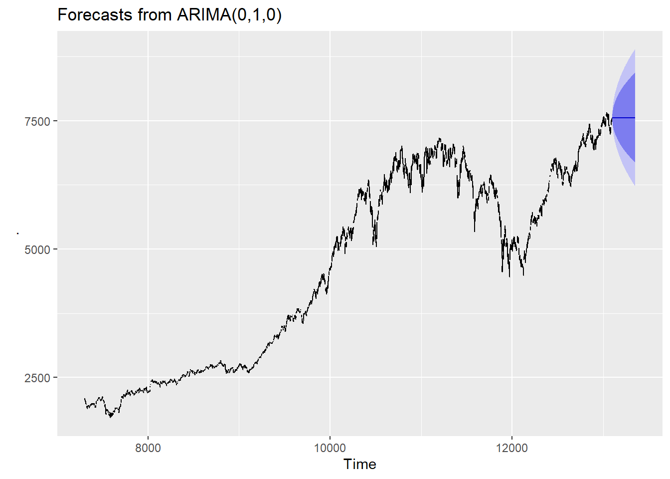

The population series \(pop\) in the wooldridge::consump dataset has an extremely small amount of volatility, so longer run forecasts are predicted with much smaller error. This data set has 37 observations of annual data from 1959 to 1995, but because the volatility is so low, we get a tight error band for long term forecasts.

consump2 <- ts(consump, start = 1959, frequency = 1)

consump2[ ,"pop"] %>% 
  auto.arima() %>% 
  forecast(h = 37) %>% 
  autoplot()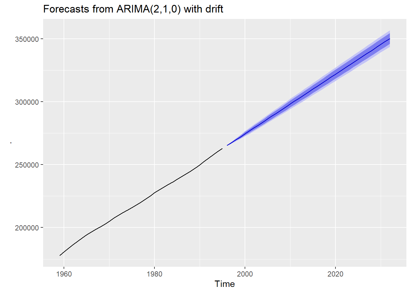

Given that the data is so old, we may wonder if they were accurate? If we rerun the code without the autoplot() call at the end, we can see what the forecasts were:

consump2[ ,"pop"] %>% 
  auto.arima() %>% 
  forecast(h = 37) 

##      Point Forecast    Lo 80    Hi 80    Lo 95    Hi 95
## 1996       265342.7 265130.0 265555.5 265017.3 265668.2
## 1997       267641.0 267141.0 268141.0 266876.3 268405.7
## 1998       269955.0 269148.8 270761.3 268722.0 271188.0
## 1999       272291.3 271201.1 273381.5 270623.9 273958.6
## 2000       274645.8 273310.0 275981.6 272602.9 276688.8
## 2001       277011.7 275468.8 278554.5 274652.1 279371.2
## 2002       279382.4 277664.4 281100.5 276754.9 282010.0
## 2003       281754.0 279884.2 283623.8 278894.5 284613.6
## 2004       284124.4 282119.3 286129.5 281057.9 287191.0
## 2005       286493.1 284363.8 288622.4 283236.7 289749.6
## 2006       288860.4 286614.7 291106.1 285426.0 292294.9
## 2007       291226.9 288870.6 293583.2 287623.2 294830.6
## 2008       293593.0 291130.6 296055.4 289827.1 297358.9
## 2009       295959.0 293394.6 298523.4 292037.1 299881.0
## 2010       298325.1 295662.3 300988.0 294252.7 302397.6
## 2011       300691.4 297933.5 303449.3 296473.6 304909.2
## 2012       303057.7 300207.9 305907.6 298699.3 307416.2
## 2013       305424.2 302485.3 308363.1 300929.5 309918.8
## 2014       307790.6 304765.3 310815.9 303163.8 312417.4
## 2015       310157.1 307047.8 313266.4 305401.8 314912.3
## 2016       312523.5 309332.4 315714.6 307643.2 317403.8
## 2017       314889.9 311619.2 318160.7 309887.7 319892.2
## 2018       317256.4 313907.8 320605.0 312135.1 322377.6
## 2019       319622.8 316198.2 323047.4 314385.3 324860.3
## 2020       321989.2 318490.2 325488.3 316637.9 327340.5
## 2021       324355.6 320783.8 327927.5 318892.9 329818.4
## 2022       326722.1 323078.8 330365.3 321150.1 332294.0
## 2023       329088.5 325375.2 332801.8 323409.5 334767.5
## 2024       331454.9 327672.9 335236.9 325670.8 337239.0
## 2025       333821.3 329971.8 337670.8 327934.0 339708.7
## 2026       336187.7 332271.9 340103.6 330199.0 342176.5
## 2027       338554.2 334573.1 342535.3 332465.6 344642.7
## 2028       340920.6 336875.3 344965.9 334733.9 347107.3
## 2029       343287.0 339178.6 347395.5 337003.7 349570.3
## 2030       345653.4 341482.8 349824.1 339275.0 352031.9
## 2031       348019.9 343787.9 352251.8 341547.6 354492.1
## 2032       350386.3 346093.9 354678.7 343821.6 356950.9

Based on this data, the forecasted 2020 population of the US was 319.6M with an 80% interval of 318.5M to 325.5M and a 95% interval of 316.6M to 327.3M. The 2020 Census estimated a popluation of 331.4M, well outside even the 95% confidence interval. In fact, the official 2000 Census figure (281.4M) is outside of the forecasted range as well! Just because the forecast looks accurate, doesn’t mean it necessarily is.

10.7 Wrapping Up

Time series modeling is the empirical backbone of much of macroeconomics and finance. This chapter only scratched the surface of what one can do with time series; is already too long and yet it feels incomplete! Nonetheless, the next chapter combines time series analysis with cross-sectional analysis in the form of Panel Data.

10.8 End of Chapter Exercises

Time Series: For each of the following examine the data (and the help file for the data) identify time series variables to model (note that some data series may need to be transformed with the ts() function). Plot the time series, and try to guess the extent to which the series is an AR(p), I(d), and/or MA(q) series. Use the auto.arima() function to identify the order of the time series. Forecast the series. If the data is old enough, see if you can find some contemporary data to check your forecast. Finally, comment on and analyze your results. Note: if you run an auto.arima() on a time series and it tells you that it is an ARIMA(0,0,0) model, you may want to try a different variable

1. wooldridge::consump, variables to look at include \(i3\), \(inf\), \(rdisp\), \(rnondc\), \(rserv\), \(c\), and/or \(rcons\). Avoid using the lags built into the dataset.

2. AER:BenderlyZwick, either of the inflation variables.

3. AER:ChinaIncome,All variables are usable.

4. AER:DJIA8012 has daily Dow Jones data.

5. AER:TechChange