Chapter 5 Intro to Regression
Regression modeling is at the center of econometric methods. Starting here, the majority of this text will focus on either regression models or extensions of the regression model. We begin with the simplest of regressions; this chapter will focus heavily on bivariate ordinary least squares (OLS) modeling and introduce multivariate OLS.
As usual, let’s start by pre-loading most of the data we will be using in this notebook:
library(AER)
library(wooldridge)
library(fivethirtyeight)
data(CPS1985)
attach(CPS1985)
data(airfare)
data(gpa2)
data(vote1)
data(meap01)
data(wine)
data(pulitzer)
data("StrikeDuration")
5.1 Prelude to Regression: The Correlation Test
We saw how to calculate a correlation (Pearson’s r) in Chapter 3. Using the CPS1985 data, we can calculate the correlation between wage and years of education using cor() function:
cor(wage, education)## [1] 0.3819221Pearson’s r looks at the strength of the linear relationship between two variables; graphically, it looks something like this:
CPS1985 %>% ggplot(aes(x = education, y = wage)) +
    geom_point() +
    geom_smooth(method = lm)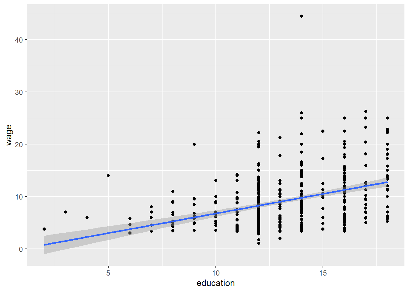
The correlation is a measure of the strength on the linear relationship between the x variable (education) and the y variable (wage). If the correlation coefficient were 1, we could say that these variables had a perfect positive linear relationship, If it were 0, we would say that these variables are unrelated. The correlation test allows us to ask if .38 is statistically significant?
- \(H_0\): The true correlation coefficient is 0, \(\rho=0\)
- \(H_1\): The true correlation coefficient is not 0, \(\rho \ne 0\)
We can test this hypothesis with the function cor.test():
cor.test(education, wage)##
## Pearson's product-moment correlation
##
## data: education and wage
## t = 9.5316, df = 532, p-value < 2.2e-16
## alternative hypothesis: true correlation is not equal to 0
## 95 percent confidence interval:
## 0.3070208 0.4521212
## sample estimates:
## cor
## 0.3819221This indicates that the correlation coefficient is in fact significantly different from 0.
Let’s look at the correlation between years of experience and wage. Again, it is useful to start by looking at a graph of the data:
CPS1985 %>% ggplot(aes(x = experience, y = wage)) +
geom_point() +
geom_smooth(method = lm)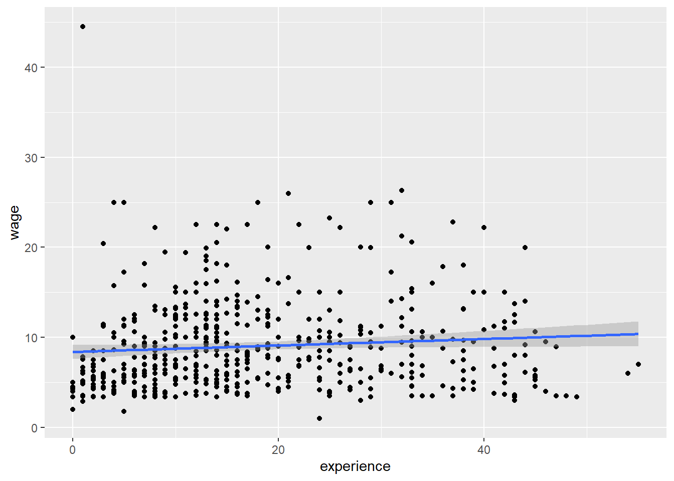 This looks a lot like a horizontal line, indicating there is probably no relationship between experience and wage. Let’s run the test, just to be sure:
cor.test(wage, experience)##
## Pearson's product-moment correlation
##
## data: wage and experience
## t = 2.0157, df = 532, p-value = 0.04433
## alternative hypothesis: true correlation is not equal to 0
## 95 percent confidence interval:
## 0.002225287 0.170649603
## sample estimates:
## cor
## 0.08705953The p-value is 0.044, which is barely less than 0.05. So again we reject the null hypothesis. Perhaps it is a good thing we ran the test rather than simply look at the graph!
Another type of correlation is the Spearman correlation; typically, you might want to use the Spearman test rather than the Pearson test if you have skewed data or outliers. Looking at the graph, it’s probably the case that income data is skewed right:
CPS1985 %>% ggplot(aes(x = wage)) +
    geom_histogram(binwidth = 2)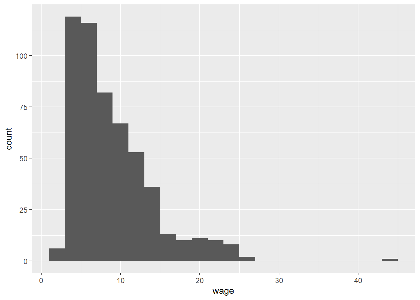
So let’s take a look at the Spearman test results:
cor.test(wage, experience, method = "spearman", exact = FALSE)##
## Spearman's rank correlation rho
##
## data: wage and experience
## S = 21090506, p-value = 8.718e-05
## alternative hypothesis: true rho is not equal to 0
## sample estimates:
## rho
## 0.1689713The Spearman statistic \(\rho = 0.17\) is significantly different from 0. Because this data is skewed, the Spearman statistic is probably more accurate than the Pearson.
5.2 Ordinary Least Squares
The most basic regression model is referred to as Ordinary Least Squares, or OLS. As this model forms the basis of all that is to follow in this class, it is worth spending some time to develop a good intuition of what is going on here. It is easiest to start with the bivariate model, as we can develop the intuition graphically as well as mathematically.
In a simple, bivariate OLS, we are looking at the linear relationship between our dependent variable and one independent variable. Suppose we are looking at the relationship between years of education and wages, where education is our independent variable, X, and wages are our dependent variable, Y. To say this model is linear implies that the relationship between X and Y looks like:
\[\begin{equation} Y_{i} = \alpha + \beta X_{i} \end{equation}\]
That is, for any value of \(X_i\), years of education, you can determine that person’s wage by multiplying their years of education by \(\beta\) and then adding \(\alpha\). We can display this graphically as well. In the graph below, assume that the \(X\) axis measures years of education and the \(Y\) axis captures wages. Graphically, this relationship looks like:
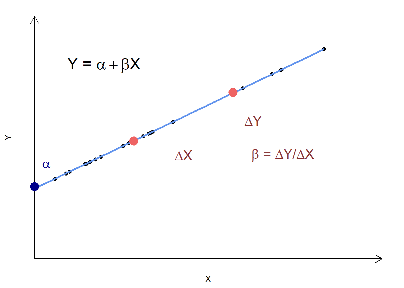
If each of the black dots represents a person, this is an example of a model that is fully determined – there is no scope for individuals to not be on the line. If, for example, \(\beta = 1\) and \(\alpha = 0.5\), then we would say that someone with 7 years of education should have an hourly wage of $7.50, someone with 13 years an hourly wage of $13.50, and so forth.
The real world is rarely so neat and tidy, and a regression is an example of a stochastic model. In a stochastic model, we use statistical tools to approximate the line that best fits the data. That is, we are still trying to figure out what \(\alpha\) and \(\beta\) are, but we are aware that not everybody will be on the line that is implied by \(\alpha\) and \(\beta\). This means that the model looks more like:
\[\begin{equation} Y_{i} = \alpha + \beta X_{i} + \epsilon_i \end{equation}\]
The new term, \(\epsilon_i\), is called the error term or the residual. Where does the error term come from? We take our values of and and combine them with \(X_i\) to calculate a predicted value of Y. Typically we refer to the predicted value of Y as \(\hat{Y}\) (pronounced Y-hat). The difference between the actual value of \(Y_i\) and \(\hat{Y}\) is \(\epsilon_i\):
\[\begin{equation} \epsilon_{i} = \hat{Y} - Y_i \end{equation}\]
The theory (and math) behind a regression model focuses on trying to estimate values for \(\alpha\) and \(\beta\) that best fits the observed data. Because we don’t know \(\alpha\) and \(\beta\), we estimate \(\hat{\alpha}\) and \(\hat{\beta}\) with our regression.
In a regression model, we estimate a model that looks like:
\[\begin{equation} Y_{i} = \hat{\alpha} + \hat{\beta} X_{i}+ \epsilon_{i} \end{equation}\]
In this model, \(\epsilon_i\) is referred to as our residual, which is just the vertical distance each individual data point is from the line implied by \(\hat{\alpha}\) and \(\hat{\beta}\).
Perhaps this is easier to understand if looked at graphically:
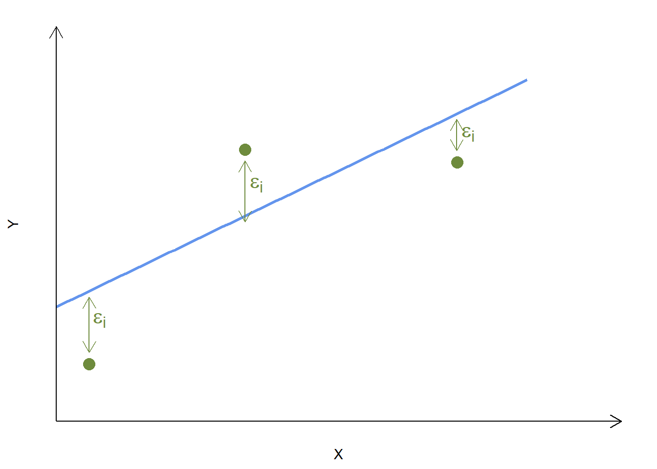
Assume that the blue line is the one implied by our estimates of \(\hat{\alpha}\) and \(\hat{\beta}\), and each green point represents one of our data poins. The vertical distance each point is from the line is its residual \(\epsilon_i\).
So where do \(\hat{\alpha}\) and \(\hat{\beta}\) come from? In other words, how do we determine the line of best fit?
The best fitting line is the one where the values of \(\hat{\alpha}\) and \(\hat{\beta}\) minimize the sum of squared errors, \(\Sigma{\epsilon_i^2}\). This is why the method is called Ordinary Least Squares! In principle, we could take a data set, run it through every single possible combination of \(\hat{\alpha}\) and \(\hat{\beta}\), calculate, square, and sum all the values of \(\epsilon_i\) that result from those values of \(\hat{\alpha}\) and \(\hat{\beta}\), and choose the \(\hat{\alpha}\) and \(\hat{\beta}\) that minimize \(\Sigma{\epsilon_i^2}\). While this method would work, it would be incredibly time (and computer memory) intensive. There is a much cleaner way of doing this, but it involves a fair bit of calculus and matrix algebra. As the focus of this book is applied economietrics, this math will be left as an exercise for the interested student to research on his/her own.
5.3 Estimating and Interpreting a Bivariate Regression
Now that we have seen some of the graphical intuition going on behind the scenes of a regression, let us proceed to estimating a regression using R and interpreting the results.
5.3.1 Estimating the Model
Let’s look again at the CPS1985 dataset and the relationship between education and wage. Again, the scatter plot looks like:
CPS1985 %>% ggplot(aes(x = education, y = wage)) +
geom_point() 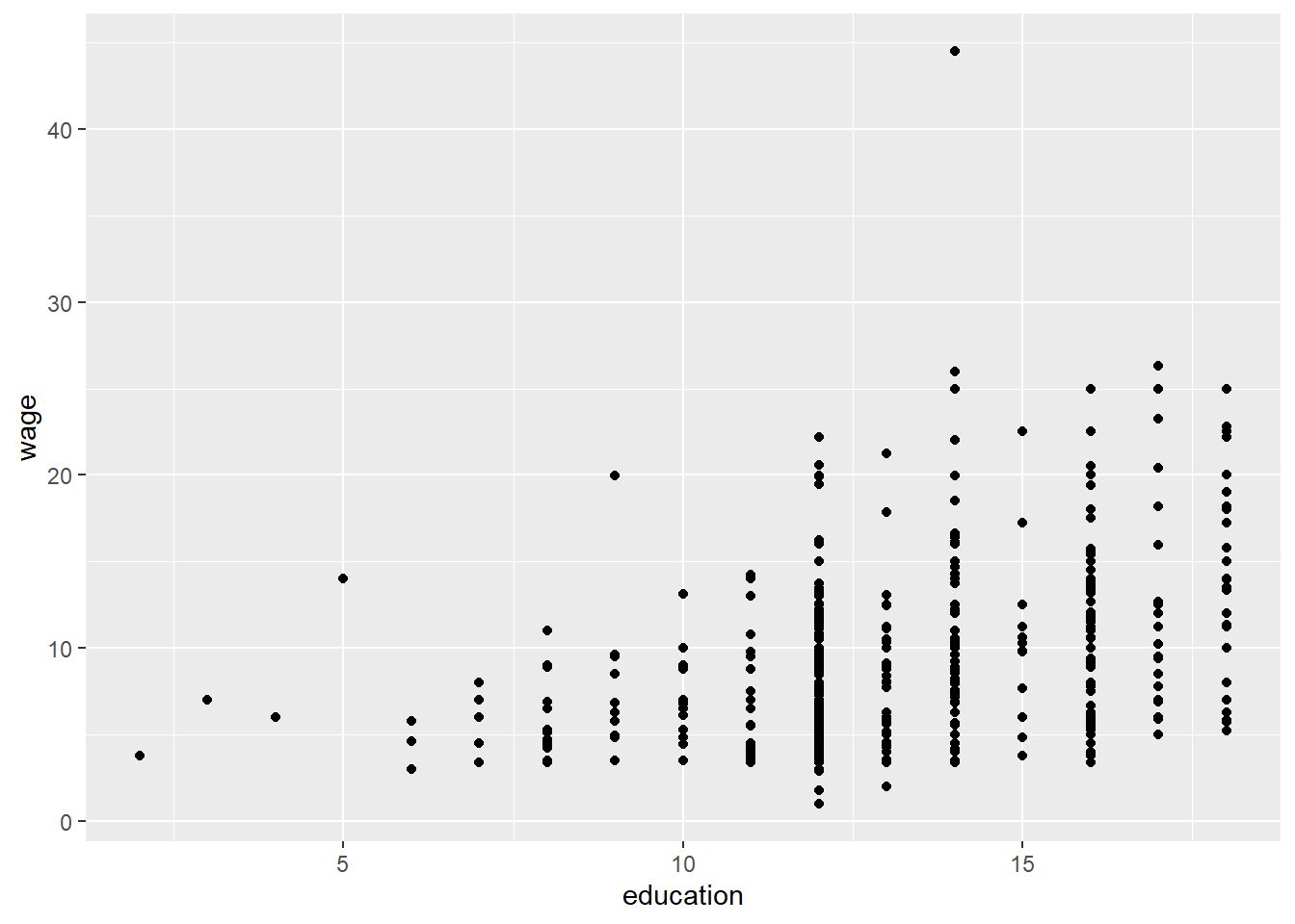
We can estimate a regression model between wage and education with the lm() command. If it helps you remember the command, lm() stands for linear model. Because we attached the CPS1985 dataset, we could simply use the command lm(wage ~ education) if we wanted, but here I will explicitly tell R which data to use.
lm(wage ~ education, data = CPS1985)##
## Call:
## lm(formula = wage ~ education, data = CPS1985)
##
## Coefficients:
## (Intercept) education
## -0.7460 0.75055.3.2 Obtaining Useful Results
As seen above, the immediate output from a regression model is not very helpful; it tells you the values of \(\hat{\alpha}\) and \(\hat{\beta}\) – these are the coefficients of the model – but that’s it. You pretty much always want to store your model as an object and inspect the object separately.
reg1 <- lm(wage ~ education, data = CPS1985)We can use the attributes() command to see what is contained within this object; we will make use of some of these shortly.
attributes(reg1)## $names
## [1] "coefficients" "residuals" "effects" "rank"
## [5] "fitted.values" "assign" "qr" "df.residual"
## [9] "xlevels" "call" "terms" "model"
##
## $class
## [1] "lm"To interpret the model, we need to take a deeper look at this regression object. The Base R method is to use the summary() command, though I prefer stargazer because it’s cleaner and the format looks like the way regressions get published in academic journals. Unfortunately, stargazer does not work for all the methods we will cover in this book, so for more some of the more advanced applications later in the text we will make use of the export_summs() command in the jtools package. Configuring export_summs() is more complex, so whenever possible we will stick with stargazer.
summary(reg1)##
## Call:
## lm(formula = wage ~ education, data = CPS1985)
##
## Residuals:
## Min 1Q Median 3Q Max
## -7.911 -3.260 -0.760 2.240 34.740
##
## Coefficients:
## Estimate Std. Error t value Pr(>|t|)
## (Intercept) -0.74598 1.04545 -0.714 0.476
## education 0.75046 0.07873 9.532 <2e-16 ***
## ---
## Signif. codes: 0 '***' 0.001 '**' 0.01 '*' 0.05 '.' 0.1 ' ' 1
##
## Residual standard error: 4.754 on 532 degrees of freedom
## Multiple R-squared: 0.1459, Adjusted R-squared: 0.1443
## F-statistic: 90.85 on 1 and 532 DF, p-value: < 2.2e-16stargazer(reg1, type = "text")##
## ===============================================
## Dependent variable:
## ---------------------------
## wage
## -----------------------------------------------
## education 0.750***
## (0.079)
##
## Constant -0.746
## (1.045)
##
## -----------------------------------------------
## Observations 534
## R2 0.146
## Adjusted R2 0.144
## Residual Std. Error 4.754 (df = 532)
## F Statistic 90.852*** (df = 1; 532)
## ===============================================
## Note: *p<0.1; **p<0.05; ***p<0.01These displays are a lot more useful. There’s lots of stuff in these outputs. The values of \(\hat{\alpha}\) and \(\hat{\beta}\) are found in the coefficients panel–the estimate of the Intercept/constant is \(\hat{\alpha}\) and the estimated coefficient on education is \(\hat{\beta}\). This means that our regression model is in fact:
\[\begin{equation} \hat{Wage_{i}} = -0.74598 + 0.75046 Education_{i} \end{equation}\]
5.3.3 Predicted Values and Residuals
We can use this equation to make predictions: the predicted wages of somebody with 12 years of education is:
\[\begin{equation} \hat{Wage_{i}} = -0.74598 + 0.75046 * 12 \end{equation}\]
\[\begin{equation} \hat{Wage_{i}} = \$8.26 \end{equation}\]
If there was a person in the dataset with 12 years of education and a wage of $8.26, their residual, \(\epsilon_i\), would be zero because the predicted value of their wage, \(\hat{Y}\), would equal their actual wage \(Y\). If their actual wage was anything other than $8.26, they would have a residual associated with them equal to \(Y-\hat{Y}\). For example, an individual with 12 years of education and an actual income of $7.50 would have an \(\epsilon_i=7.50-8.26=-0.76\)
In the process of running this regression, R already calculated predicted values and residuals for every single observation in the dataset! Recall above that we used the attributes(reg1) command and saw that we can grab the model’s residuals, \(\epsilon_i\), and fitted values, \(\hat{Y_i}\). This next code clones the CPS1985 data into a new dataset called tempdata, attaches the residuals and fitted values to that new dataset, and gets rid of all the variables we didn’t use in our regression. This table shows the first 10 observations in the data set, along with their predicted values and residuals:
resids <- reg1$residuals
preds <- reg1$fitted.values
tempdata <- cbind(CPS1985, preds, resids)
tempdata %>%
    select(c(wage,education, preds, resids)) %>%
    slice(1:10)
## wage education preds resids
## 1 5.10 8 5.257706 -0.1577063
## 1100 4.95 9 6.008167 -1.0581671
## 2 6.67 12 8.259549 -1.5895493
## 3 4.00 12 8.259549 -4.2595493
## 4 7.50 12 8.259549 -0.7595493
## 5 13.07 13 9.010010 4.0599899
## 6 4.45 10 6.758628 -2.3086278
## 7 19.47 12 8.259549 11.2104507
## 8 13.28 16 11.261392 2.0186076
## 9 8.75 12 8.259549 0.4904507Recall, wage is our dependent variable (\(Y\)), and education is our independent variable (\(X\)). The \(preds\) variable records the values of \(\hat{Y}\) for each level of education \(X_i\) and the \(resids\) variable records how far from the predicted wage \(\hat{Y}\) each of the actual wages \(Y_i\) is.
5.3.4 Look at the stars, look how they shine for you
As an aside, Coldplay sucks. Rather than dwell upon their excrementary music, let’s look back at the stargazer() output so we can think happy thoughts again:
stargazer(reg1, type = "text")##
## ===============================================
## Dependent variable:
## ---------------------------
## wage
## -----------------------------------------------
## education 0.750***
## (0.079)
##
## Constant -0.746
## (1.045)
##
## -----------------------------------------------
## Observations 534
## R2 0.146
## Adjusted R2 0.144
## Residual Std. Error 4.754 (df = 532)
## F Statistic 90.852*** (df = 1; 532)
## ===============================================
## Note: *p<0.1; **p<0.05; ***p<0.01You should have noticed all the stars next to the education coefficient. The the stars are very useful for interpreting the statistical significance of your regression model. In a regression, the null hypothesis is that the true coefficients (\(\beta\) and \(\alpha\)) are equal to zero, the alternative hypothesis is that they are not equal to zero. Most of the time we are not concerned with \(\alpha\) or its significance; rather, we focus on \(\beta\) and whether or not our estimate of \(\hat{\beta}\) is significantly different from zero.
Why zero? If \(\beta > 0\), higher values of \(X_i\) are associated with higher values of \(Y_i\). If \(\beta < 0\), higher values of \(X_i\) are associated with lower values of \(Y_i\). If \(\beta = 0\), then there is no relationship between our dependent variable and our independent variable. In other words, our null hypothesis is that X and Y are unrelated, and by rejecting the null hypothesis we are saying that we believe that X and Y are in fact related.
The bottom panel shows useful information about the regression. Observations is your sample size, and R2 is actually \(R^2\) (pronounced R-squared) and is a measure of goodness of fit. The possible range for\(R^2\) is \(0 \geq R^2 \geq 1\). In a bivariate model, \(R^2\) is actually the correlation coefficient squared!
cor(wage, education)## [1] 0.3819221cor(wage, education)^2## [1] 0.1458645\(R^2\) is often called the coefficient of determination, and, while not technically true, is easiest thought of as the percentage of the variation in \(Y\) that you can explain with your independent variable \(X\). Our \(R^2=0.146\) then might be interpreted as saying that we can explain roughly 15% of the variation in wages with education, and therefore the other 85% of the variation in wages is left unexplained.
The F-test is a measure of the significance of the entire model–the null hypothesis is that every \(\hat{\beta}\) that you estimated is equal to zero. In a bivariate model, there is only \(\hat{\beta}\) so the F-test of the model is basically the same thing as the t-test of \(\hat{\beta}\).
5.3.5 Visualizing the Regression Line
Using ggplot(), it is easy to add the regression line to a scatterplot to visualize the relationship. We can use geom_point() to create the scatterplot and add the regression line with the geom_smooth(method = lm) argument.
CPS1985 %>% ggplot(aes(x = education, y = wage)) +
    geom_point() +
    geom_smooth(method = lm,
                se = FALSE)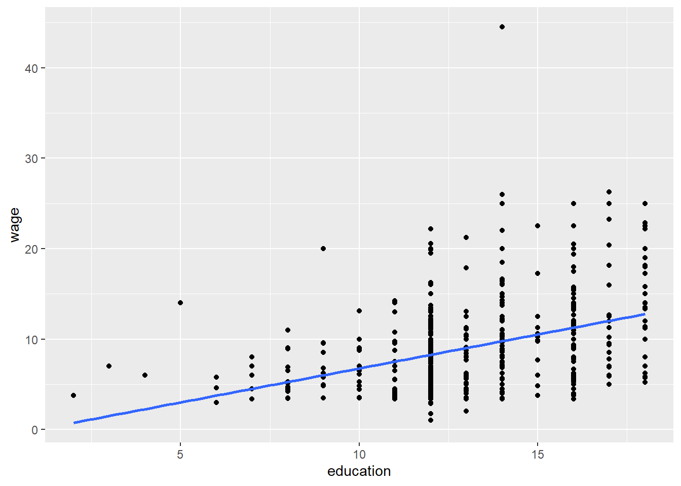
5.4 More Examples of Bivariate Regression
Now that we have the basics of regression down, let’s try running and interpreting regressions with a few more datasets. We will add more nuance to our interpretation as we go.
5.4.1 Introducing Data Transformations
Let’s start with the airfare data and examine the relationship between the average one-way fare and the distance in miles of the routes. Which variable should be dependent and which should be independent? Statistics cannot prove causation, that is the role of (economic) theory. But when constructing our regressions, we should be thinking about economic logic and how it informs our thinking about causality.

Figure 5.1: Correlation vs Causation
In this case, it is likely that distance is the cause of the price, and not the other way around, so we put distance on the X-axis and airfare on the Y-axis. We can start by looking at a scatterplot:
airfare %>% ggplot(aes(x = dist, y = fare)) +
    geom_point(size = .7) +
    geom_smooth(method=lm)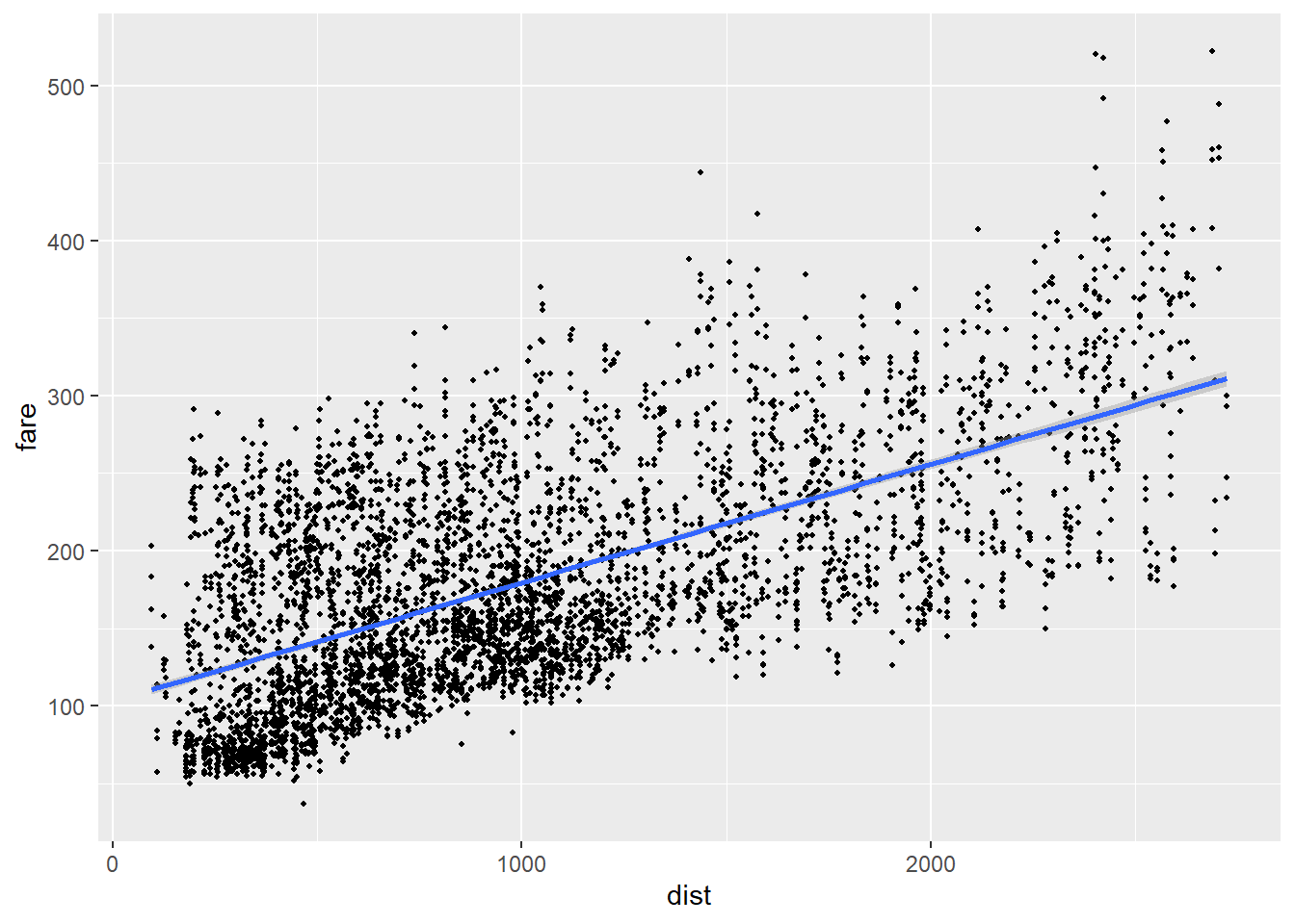
Next, we can estimate the regression model using the lm() command. Because I didn’t attach the dataset, I need to tell the lm() function where the variables are. One option would be to use the $ notation, as in lm(airfare$fare ~ airfare$dist), though I prefer the lm(fare ~ dist, data = airfare) syntax because I stopped paying attention in typing class when we got to the section on symbols and I always make typos when I type $:
reg2 <- lm(fare ~ dist, data = airfare)The regression output is stored in the object reg2, so let’s use stargazer() to check it out. The stargazer() function defaults to output in LaTeX, so you may want to stick with the type = "text" option. If you want to make prettier versions of stargazer() output to cut and paste into MS Word or the like, you might want to look into how to use the type = "HTML option and how to save stargazer() output.
stargazer(reg2, type = "text")##
## ===============================================
## Dependent variable:
## ---------------------------
## fare
## -----------------------------------------------
## dist 0.076***
## (0.001)
##
## Constant 103.261***
## (1.643)
##
## -----------------------------------------------
## Observations 4,596
## R2 0.389
## Adjusted R2 0.389
## Residual Std. Error 58.546 (df = 4594)
## F Statistic 2,922.832*** (df = 1; 4594)
## ===============================================
## Note: *p<0.1; **p<0.05; ***p<0.01The coefficient on the distance variable is significant at the 99% level and \(R^2 = .39\), both of which indicate strong statistical significance. Let’s think about what this means in terms of our regression equation:
\[\begin{equation} fare_{i} = 103.261 + 0.076 distance_{i} \end{equation}\]
The \(\beta\) implies that, if distance increases by 1, fare increases by 0.076. What are the units of measure here? Distance is measured in miles, and fare is measured in $US. So this equation suggests that, on average, a one mile increase in the distance of a flight is associated with a $0.076 (7.6 cent) increase in price. This isn’t really an intuitive unit of measure–it may be more intuitive to think of a 100 mile increase in distance as associated with a $7.60 increase in price.
Let’s take this logic a little further and start to learn a bit about data transformation.
airfaretemp <- airfare %>%
    select(fare, dist) %>%
    mutate(dist100 = dist/100)
airfaretemp[c(1,5,9,13,17),]
## fare dist dist100
## 1 106 528 5.28
## 5 104 861 8.61
## 9 207 852 8.52
## 13 243 724 7.24
## 17 119 1073 10.73This bit of code creates a new dataset called airfaretemp and adds a new variable called dist100. The variable dist100 is created by dividing the dist variable by 100, so really it’s just measuring distance in hundreds of miles. I also had R spit out 5 lines of data just to confirm the relationship between the variables \(dist100=\frac{dist}{100}\). Now, let’s estimate the regression between fare and dist100 and put it side by side with our original regression:
reg2a <- lm(fare ~ dist100, data = airfaretemp)
stargazer(reg2, reg2a, type = "text")
##
## ============================================================
## Dependent variable:
## ----------------------------
## fare
## (1) (2)
## ------------------------------------------------------------
## dist 0.076***
## (0.001)
##
## dist100 7.632***
## (0.141)
##
## Constant 103.261*** 103.261***
## (1.643) (1.643)
##
## ------------------------------------------------------------
## Observations 4,596 4,596
## R2 0.389 0.389
## Adjusted R2 0.389 0.389
## Residual Std. Error (df = 4594) 58.546 58.546
## F Statistic (df = 1; 4594) 2,922.832*** 2,922.832***
## ============================================================
## Note: *p<0.1; **p<0.05; ***p<0.01This is pretty cool–the results are more or less identical, except for the decimal places with respect to the distance variable and its standard error. And we get the same intuitive result we saw above.
5.4.2 Does Alpha Matter?
Next, let’s take a look at the gpa2 data. This data includes student data from a midsize research university. Let’s look at the relationship between a student’s SAT score and his/her GPA after the fall semester:
gpa2 %>%  ggplot(aes(x = sat, y = colgpa)) +
    geom_point(size = .7) +
    geom_smooth(method = lm) +
  labs(y = "GPA",
       x = "SAT Score") +
  theme_classic()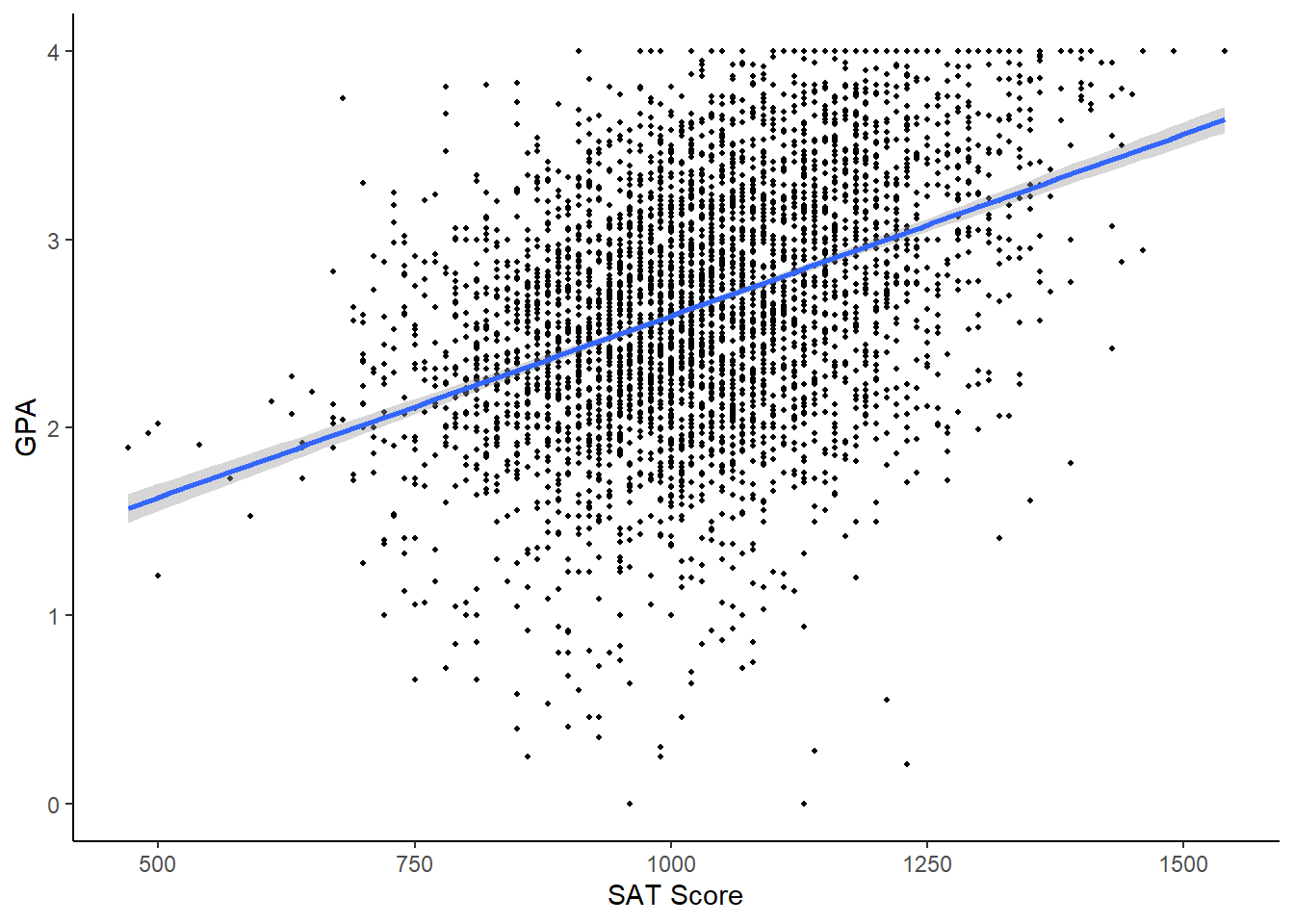
Next, store the regression in an object and look at it using stargazer()
reg3 <- lm(colgpa ~ sat, data = gpa2)
stargazer(reg3, type = "text")
##
## ===============================================
## Dependent variable:
## ---------------------------
## colgpa
## -----------------------------------------------
## sat 0.002***
## (0.0001)
##
## Constant 0.663***
## (0.070)
##
## -----------------------------------------------
## Observations 4,137
## R2 0.167
## Adjusted R2 0.167
## Residual Std. Error 0.601 (df = 4135)
## F Statistic 829.258*** (df = 1; 4135)
## ===============================================
## Note: *p<0.1; **p<0.05; ***p<0.01Here, \(R^2 = .17\) and our estimate of \(\hat{\beta}\) is significant at the 99% level. We can interpret the coefficient of .002 as stating that we expect GPA go go up by .002 on average for every 1 point of SAT. This is a bit of an awkward interpretation, notably because SAT scores don’t go up by 1, they go up by 10! We can use the same trick as above to scale these numbers in a way that is more meaningful; a 100 point increase in overall SAT score is associated with a 0.2 increase in GPA seems a lot more meaningful.
Let’s look at the estimated value of \(\hat{\alpha}\) of 0.663. What does that mean, and what does it mean that it is significant? Let’s start with the question of what it means and look at the regression equation:
\[\begin{equation} gpa_{i} = 0.663 + 0.002 sat_{i} \end{equation}\]
What would our expected gpa, \(\hat{gpa}\), be for a student who earned a 0 on the SAT? Anything multiplied by 0 is 0, so 0.663 is our estimated GPA for somebody who earned a 0 on the SAT. But is it even possible to earn a 0 on the SAT? They give you 400 points just for showing up alive. So looking at a 0 on the SAT is somewhat meaningless in this model, because it is impossible to even get. The \(\alpha\) in the equation is valuable for calculating predicted values, but in most cases, \(\hat{\alpha}\) is not really what we are looking at in a regression model. This brings us to the question of the significance of the \(\hat{\alpha}\) term - the fact that we are pretty darn sure that the true value of \(\alpha\) is not really 0 doesn’t really mean anything here.
5.4.3 Alternative Hypothesis Tests
Most of the time, the value of \(\hat{\alpha}\) is not of terrible importance, though here is a counterexample: consider the CAPM model, a standard model in finance. The CAPM model can be written as:
\[\begin{equation} (R-R_f)=\alpha + \beta(R_m-R_f) \end{equation}\]
Where:
- \(R\) is the rate of return of an asset or portfolio
- \(R_f\) is the risk-free rate of return
- \(R_m\) is the market rate of return
- \(\beta\) is the relative volatility of the asset
- \(\alpha\) is a risk-adjusted rate of return: the extent to which the asset under- or over-performed the market when taking into consideration the riskiness of the asset
The CAPM model can be estimated using bivariate regression, and when people in finance talk about stock market betas, they are literally talking about \(\beta\) from a CAPM regression! In this model, you may in fact not only be interested to know the value of \(\alpha\), but whether or not it is significantly different from zero is of importance as well!
Getting the data for this will be a bit tricky; to follow along you will need to install the tidyquant and quantmod packages:
firstsolar <- tq_get('FSLR', # firstsolar Ticker
               from = "2017-01-01",
               to = "2018-01-01",
               get = "stock.prices")
vanguard500 <- tq_get('VFINX',  # vanguard500 Ticker
               from = "2017-01-01",
               to = "2018-01-01",
               get = "stock.prices")
coke <- tq_get('KO',  # Coke Ticker
               from = "2017-01-01",
               to = "2018-01-01",
               get = "stock.prices")
spx <- tq_get('^GSPC',  # S&P 500 Ticker
               from = "2017-01-01",
               to = "2018-01-01",
               get = "stock.prices")
tbill <- tq_get('^IRX', # 90 day T-bill
               from = "2017-01-01",
               to = "2018-01-01",
               get = "stock.prices")
# Convert stocks prices into daily rates of return
firstsolar <- firstsolar %>%
    select(date, adjusted) %>%
    mutate(lnadjusted = log(adjusted)) %>%
    mutate(firstsolar = lnadjusted - lag(lnadjusted)) %>%
    select(date, firstsolar)
vanguard500 <- vanguard500 %>%
    select(date, adjusted) %>%
    mutate(lnadjusted = log(adjusted)) %>%
    mutate(vanguard500 = lnadjusted - lag(lnadjusted)) %>%
    select(date, vanguard500)
coke <- coke %>%
    select(date, adjusted) %>%
    mutate(lnadjusted = log(adjusted)) %>%
    mutate(coke = lnadjusted - lag(lnadjusted)) %>%
    select(date, coke)
spx <- spx %>%
    select(date, adjusted) %>%
    mutate(lnadjusted = log(adjusted)) %>%
    mutate(spx = lnadjusted - lag(lnadjusted)) %>%
    select(date, spx)
# t bill quotes are annualized, convert to daily
tbill <- tbill %>%
    select(date, adjusted) %>%
    mutate(tbill = adjusted/360) %>%
    select(date, tbill)
# Combine all the datasets
returns <- spx
returns <- merge(returns, vanguard500, by = "date")
returns <- merge(returns, firstsolar, by = "date")
returns <- merge(returns, coke, by = "date")
returns <- merge(returns, tbill, by = "date")
returns <- drop_na(returns)
I’ve attempted to document the code to help with readability. This downloads stock ticker data for First Solar (FSLR), Vanguard 500 (VFINX), Coca-Cola (KO), and S&P 500 (SPX), and the 3 month T-bill rate (which will be used for our risk-free rate).
Next, we estimate 3 CAPM regressions; one for Coke, one for First Solar, and one for the Vanguard 500, and display them in stargazer().
capm1 <- lm(coke-tbill~spx-tbill, data = returns)
capm2 <- lm(firstsolar-tbill~spx-tbill, data = returns)
capm3 <- lm(vanguard500 - tbill ~ spx - tbill, data = returns)
stargazer(capm1, capm2, capm3, type = "text")
##
## ==================================================================================
## Dependent variable:
## ---------------------------------------------------
## coke - tbill firstsolar - tbill vanguard500 - tbill
## (1) (2) (3)
## ----------------------------------------------------------------------------------
## spx
##
##
## Constant -0.003*** -0.003*** -0.003***
## (0.00004) (0.00004) (0.00004)
##
## ----------------------------------------------------------------------------------
## Observations 251 251 251
## R2 0.000 0.000 0.000
## Adjusted R2 0.000 0.000 0.000
## Residual Std. Error (df = 250) 0.001 0.001 0.001
## ==================================================================================
## Note: *p<0.1; **p<0.05; ***p<0.01This is a model that we actually care about the value of \(\alpha\), which represents the risk-adjusted rate of return. This suggests that both coke and the Vanguard 500 had significantly negative alphas. In actuality, this is probably not true–the asset returns are calculated daily but the risk adjusted return used is a 3 month return–it would be better to have data with matching time horizons, but I digress.
It might also be of note here that the significance test of our estimated \(\hat{\beta}\) values is relative to \(\beta = 0\), but in this particular application of financial econometrics, you may not be interested in \(\beta = 0\), you may be more interested in a hypothesis of whether or not the asset has equal volatility to the market (\(\beta=1\)), or if it is more (\(\beta>1\)) or less (\(\beta<1\)) volatile than the market. In finance, negative betas are theoretically possible but highly unlikely; an asset with a negative beta would be considered to be a hedge and would tend to do better when the market declines, but do worse when the market appreciates.
The easiest way to get insight into this question is to use the confint command to generate a confidence interval for the regression model:
confint(capm1) # Coke Model## 2.5 % 97.5 %
## (Intercept) -0.002643787 -0.002478988
## spx NA NAWe see that our confidence interval for our first regression (for Coca-Cola stock) states that we are 95% confident that \(-0.005<\beta<.336\), indicating that we are fairly certain that Coca-Cola stock is far less volatile than the market as a whole. Repeating this process for the First Solar stock and the Vanguard 500 fund:
confint(capm2) # First Solar Model## 2.5 % 97.5 %
## (Intercept) -0.002643787 -0.002478988
## spx NA NAconfint(capm3) # Vanguard Model## 2.5 % 97.5 %
## (Intercept) -0.002643787 -0.002478988
## spx NA NAWe see that the 95% confidence interval in the First Solar regression is \(1.229<\beta<2.873\), indicating that the finding that this stock is more volatile than the market is statistically significant at the 95% level, and we see that, unsurprisingly, the Vanguard regression shows \(0.981<\beta<1.020\) so \(\hat{\beta}\) is not significantly different from 1.
5.4.4 Not All Regressions Have Significant Results
Let’s return to some simpler examples, starting with the meap01 data; this data has school level funding and test score data in the state of Michigan. Does spending per student lead to better performing students? We can look at the relationship between the variable math4, the percent of students receiving a satisfactory 4th grade math score, and exppp, expenditures per pupil. We start by looking at a plot of the data:
meap01 %>% ggplot(aes(x = exppp, y = math4)) +
    geom_point(color = "darkslateblue",
               alpha = .6) +
    geom_smooth(method = lm)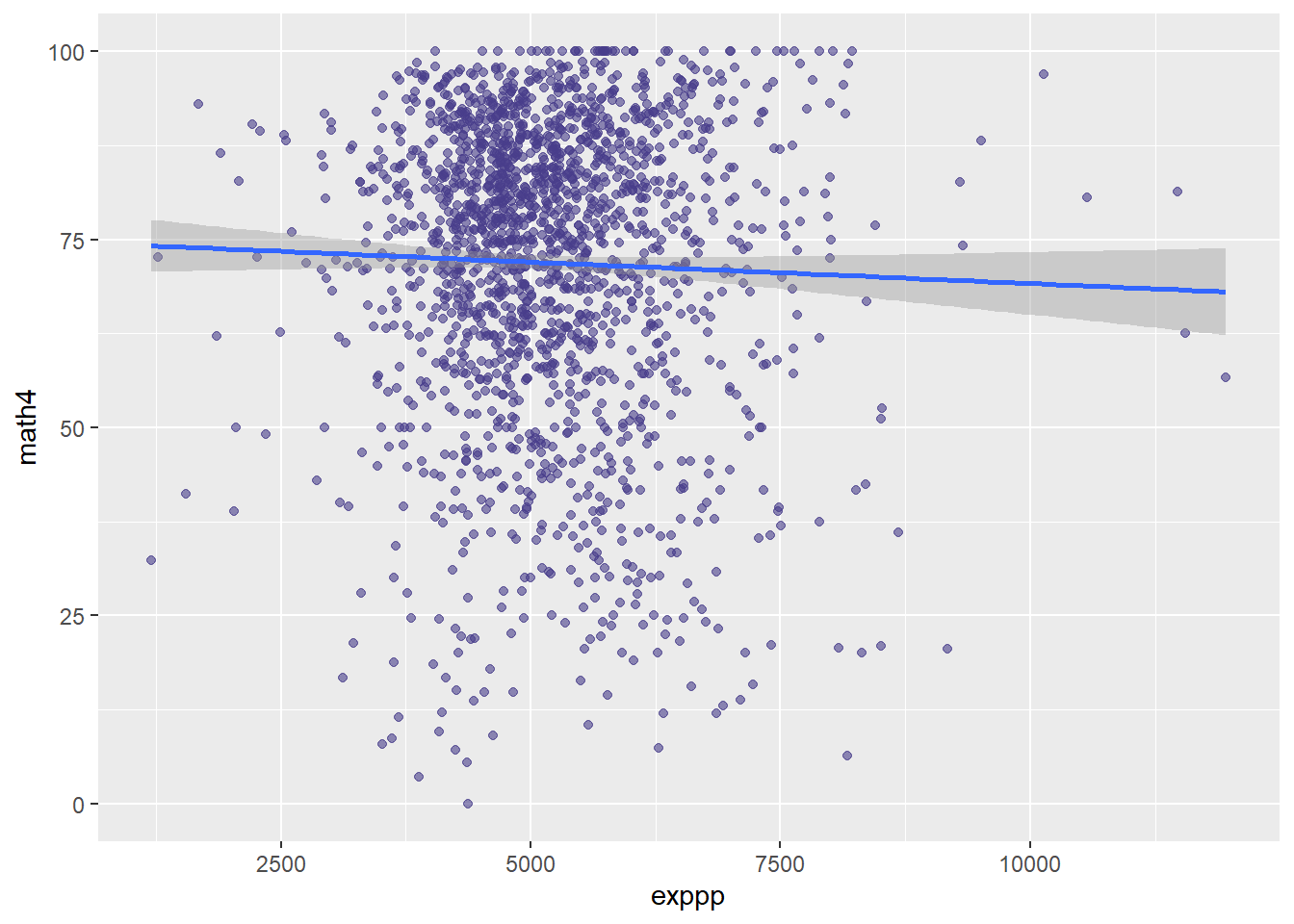
If you have read a paper or two in the economics of education literature, the slope of that line shouldn’t come as a surprise to you. Let’s estimate a regression:
reg4 <- lm(math4 ~ exppp, data = meap01)
stargazer(reg4, type  = "text")
##
## ===============================================
## Dependent variable:
## ---------------------------
## math4
## -----------------------------------------------
## exppp -0.001
## (0.0004)
##
## Constant 74.870***
## (2.272)
##
## -----------------------------------------------
## Observations 1,823
## R2 0.001
## Adjusted R2 0.0004
## Residual Std. Error 19.950 (df = 1821)
## F Statistic 1.773 (df = 1; 1821)
## ===============================================
## Note: *p<0.1; **p<0.05; ***p<0.01The sign on the \(\hat{\beta}\) is negative, which corresponds to the downward sloping line in the plot. However, there are no stars next to the coefficient, implying that the result is not significantly different from 0; thus, even though \(\hat{\beta} < 0\), we do not reject the null hypothesis that \(\beta = 0\).
5.4.5 Signs, Signs, Everywhere There’s Signs
Finally, let’s take a look at the voting data in the vote1 dataset. Specifically, let’s examine the relationship between the share of campaign expenditures (shareA) a candidate made and the vote share received (voteA). We can start with a graph:
vote1 %>% ggplot(aes(x = shareA, y = voteA)) +
    geom_point(color="indianred") +
    geom_smooth(color = "dodgerblue", method = lm, se = FALSE) +
  labs(y = "Vote Share",
       x = "Campaign Spending") +
  theme_classic()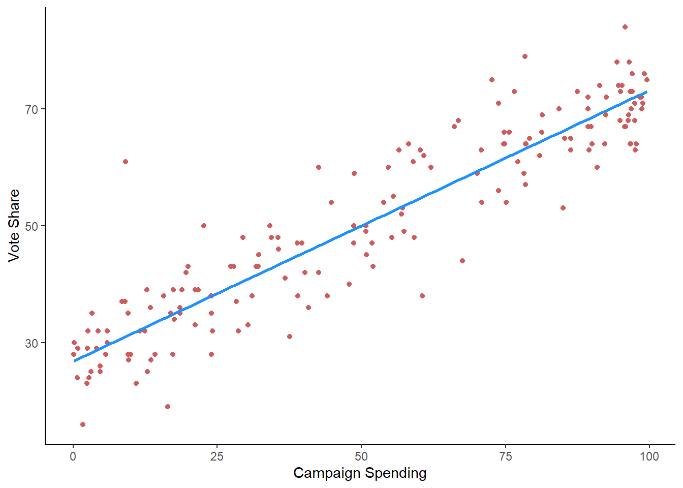
Next, we estimate the regression and put the results into stargazer() for ease of viewing.
reg5 <- lm(voteA ~ shareA, data = vote1)
stargazer(reg5, type = "text")
##
## ===============================================
## Dependent variable:
## ---------------------------
## voteA
## -----------------------------------------------
## shareA 0.464***
## (0.015)
##
## Constant 26.812***
## (0.887)
##
## -----------------------------------------------
## Observations 173
## R2 0.856
## Adjusted R2 0.855
## Residual Std. Error 6.385 (df = 171)
## F Statistic 1,017.663*** (df = 1; 171)
## ===============================================
## Note: *p<0.1; **p<0.05; ***p<0.01The \(R^2\) is pretty huge \(R^2 = 0.86\) and the \(\hat{\beta}\) is positive and significant at the 99% level. This is a tricky \(\beta\) to interpret, because the variable shareA is defined as \(\frac{Expenditures\:by\: Candiate\:A}{Expenditures\:by\:Candidate\:A + Expenditures\:by\:Candidate\:B}\). It can be done, but it is tricky. In some cases, it is easier just interpreting the signs and significance of the coefficients, and not focusing so much on the actual magnitude of the coefficients.
5.5 Multivariate Regression
We can extend this logic into having multiple independent variables. Multivariate regression is a bit harder to wrap one’s mind around, because it is really difficult to graph (adding variables adds dimensions to the graph, so we are no longer dealing with a 2d space), but the basics of interpreting the variables is the same as with bivariate modeling.
Let’s start with a basic example. Using the CPS1985 data, what happens when we include education AND age in the same regression.
reg1 <- lm(wage ~ education, data = CPS1985)
reg6 <- lm(wage ~ age, data = CPS1985)
reg7 <- lm(wage ~ education + age, data = CPS1985)
stargazer(reg1, reg6, reg7, type = "text")
##
## ===========================================================================================
## Dependent variable:
## -----------------------------------------------------------------------
## wage
## (1) (2) (3)
## -------------------------------------------------------------------------------------------
## education 0.750*** 0.821***
## (0.079) (0.077)
##
## age 0.078*** 0.105***
## (0.019) (0.017)
##
## Constant -0.746 6.167*** -5.534***
## (1.045) (0.723) (1.279)
##
## -------------------------------------------------------------------------------------------
## Observations 534 534 534
## R2 0.146 0.031 0.202
## Adjusted R2 0.144 0.029 0.199
## Residual Std. Error 4.754 (df = 532) 5.063 (df = 532) 4.599 (df = 531)
## F Statistic 90.852*** (df = 1; 532) 17.199*** (df = 1; 532) 67.210*** (df = 2; 531)
## ===========================================================================================
## Note: *p<0.1; **p<0.05; ***p<0.01As you can see, adding another variable to a lm() is incredibly easy.
The first column has the first regression in this chapter. The second looks at the relationship between age and wage, and the third column looks at the model with both education and age. First, a couple comments on interpreting the multivariate results.
We interpret the coefficients in the same way as in a bivariate model - column 3 implies that a 1 year increase in education is associated with a $0.82 increase in hourly wage, and a 1 year increase in age is associated with a $0.11 increase in wage. It is always useful to keep in mind the economic notion of ceteris parebus here!
We can make predictions the same way as well. If somebody has 16 years of education and is 34 years old, the model predicts that their wage will be \(-\$5.53 + \$0.82(16) + \$0.11(34) = \$11.33\). Even if a variable is not significant, we need to include it in our math to make predictions.
Something you may have noticed is that there is are some interesting changes from the bivariate models to the multivariate model. However, a multivariate regression doesn’t just do a bunch of bivariate regressions and slap those results together! What observations might we make when we consider these regressions side by side by side?
- The \(\hat{\beta}\) estimates in column 3 are not equal to those in column 1 or 2.
- The \(R^2\) in the multivariate model is larger than in either of the bivariate models.
These differences might lead to asking: if we are only focused on the relationship between two variables, why would we want to estimate a multivariate regression? For example, if we are concerned only with predicting the relationship between wages and years of education, what is the purpose of adding additional variables to our analysis? Wouldn’t they just get in the way and clutter the analysis?
It turns out to be essential to add additional variables to a model for it to be useful. As to why, it really depends on your purpose for running your regression: is your goal is ultimately prediction or hypothesis testing? Either way, nearly every application of regression is a multivariate application, but before we dig deepeer into multivariate regression, let’s take a brief digression into the difference between predictive modeling vs hypothesis testing.
5.5.1 Predictive Modeling vs Hypothesis Testing
The goal of regression analysis is typically prediction or hypothesis testing. Within the context of a typical regression model \(Y = \alpha +\beta_1X_1+\beta_2X_2+...+\beta_kX_k\):
Predictive modeling refers to a situation where your primary purpose is to predict outcome \(Y\) as accurately as possible. Statistics and data analytics tend to focus on predictive modeling.
Hypothesis testing refers to a model where your primary purpose is to predict the impact of a particular independent variable (e.g. \(X_1\)) or set of independent variables (e.g. \(X_1\), \(X_2\), and \(X_3\)) on the outcome \(Y\). Such a variable is commonly referred to as a variable of interest; that is, the whole purpose of running the regression is that we are interested in the coefficient on that variable. Economics tends to focus on hypothesis testing.
In either case, one should always include as independent variables all variables that they think might impact the value of the dependent variable, even if it is not the variable of interest.
5.5.2 Predictive modeling
For predictive modeling, the reason why should be clear–If you are trying to predict \(Y\), leaving out relevant information will ultimately lead to less precise and accurate predictions. As an example, imagine trying to predict wages using only a person’s age. Age probably matters for wages, but without knowing information like years of education, which also probably matters, your predictions are going to be less accurate.
Let’s look at this more closely, again using the CPS1985 data. Column 1 has a regression with age as the only \(X\) variable, column 2 includes both age and education.
reg6 <- lm(wage ~ age, data = CPS1985)
reg7 <- lm(wage ~ education + age, data = CPS1985)
stargazer(reg6, reg7, type = "text")
##
## ===================================================================
## Dependent variable:
## -----------------------------------------------
## wage
## (1) (2)
## -------------------------------------------------------------------
## education 0.821***
## (0.077)
##
## age 0.078*** 0.105***
## (0.019) (0.017)
##
## Constant 6.167*** -5.534***
## (0.723) (1.279)
##
## -------------------------------------------------------------------
## Observations 534 534
## R2 0.031 0.202
## Adjusted R2 0.029 0.199
## Residual Std. Error 5.063 (df = 532) 4.599 (df = 531)
## F Statistic 17.199*** (df = 1; 532) 67.210*** (df = 2; 531)
## ===================================================================
## Note: *p<0.1; **p<0.05; ***p<0.01To see which has more accurate predictions, let’s make a boxplot of the residuals of both models. Recall that the residual is equal to \(\epsilon_i=Y_1-\hat{y}\), and as \(\hat{y}\) is our predicted value, bigger values of \(\epsilon_i\) implies less accurate predictions.
a <- data.frame(Model = "Bivariate", Residual = resid(reg6))
b <- data.frame(Model = "Multivariate", Residual = resid(reg7))
residdata <- rbind(a,b)
ggplot(residdata) +
  geom_boxplot(aes(y = Residual, fill = Model))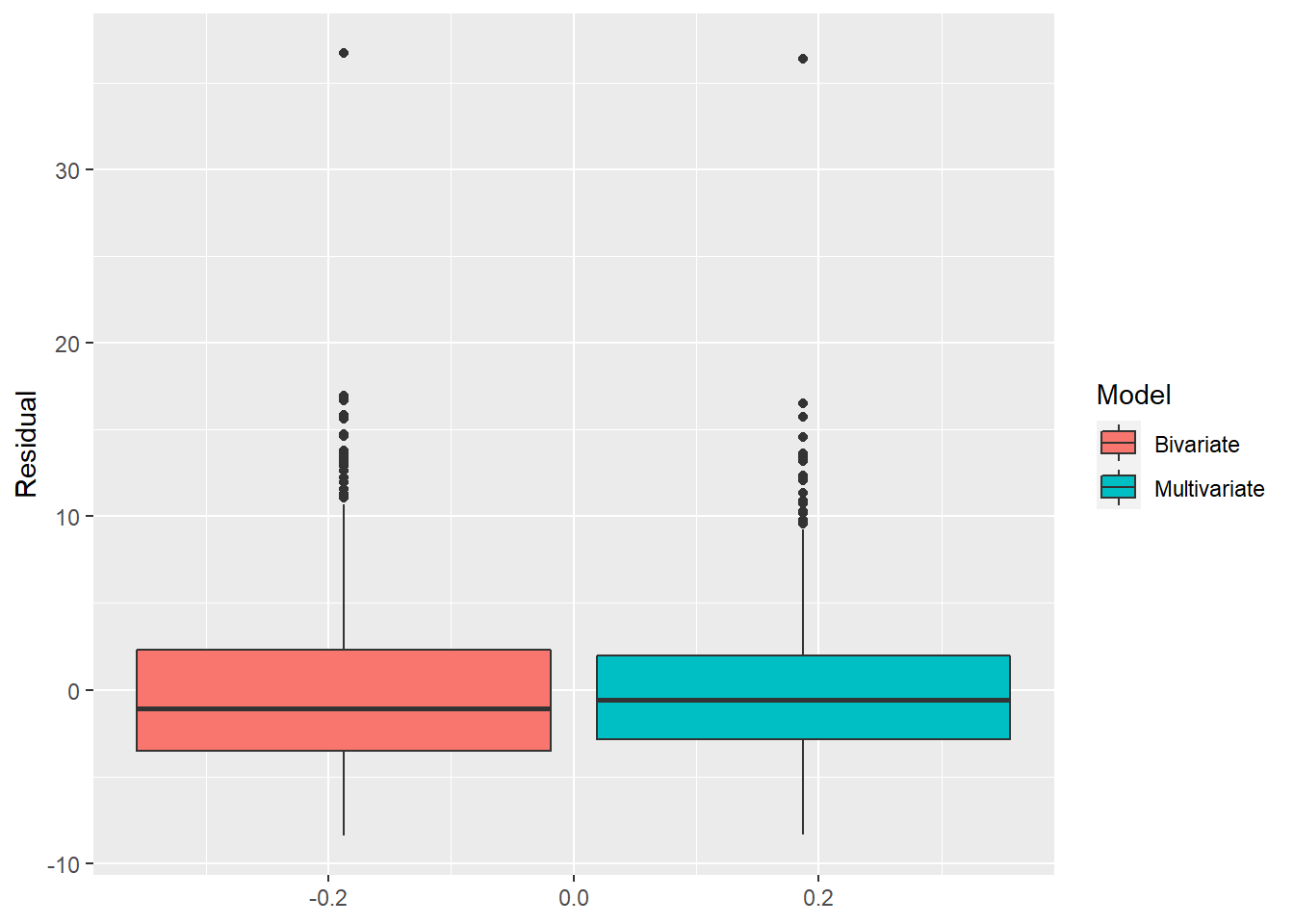
Close inspection of the two boxplots shows that the one of the right has less spread, and thus more predictive accuracy. In fact, the standard deviations of the residuals from the two models are:
sd(resid(reg6))## [1] 5.057985sd(resid(reg7))## [1] 4.590779Again we can see that the multivariate model has more predictive accuracy than the bivariate model.
5.5.3 Hypothesis testing
Hypothesis testing typically focuses on attempting to estimate the “true” relationship between one or more independent variables of interest and the dependent variable. One might naturally wonder, why worry about other variables if you are only interested in one specific \(\hat{\beta}\)? The answer lies in developing a bit deeper intuition of how the regression math works. Ordinary least squares works by attributing the variation in the dependent variable Y to the variation in your independent variables. Consider the model \(Y=\alpha +\beta X + \epsilon\): it turns out that if you go through the calculus behind OLS, you will find that \(\beta=\frac{cov(X,Y)}{var(Y)}\), an expression that basically means that \(\beta\) is calculating the extent to which variation in \(Y\) (that’s the \(var(Y)\) part) is happening jointly with the variation in \(X\) (that’s the \(cov(X,Y)\) part).
The big concern here is that maybe your variable of interest (\(X_1\)) is correlated (multicollinear) with another variable not in your model (\(X_2\)), so your estimate of \(\hat{\beta}\) will include both the direct effect of \(X_1\) and the indirect effect of \(X_2\) to the extent \(X_2\) is correlated with \(X_1\). This is referred to as omitted variable bias, which we will discuss more in Chapter 6. For the purposes of hypothesis testing, however, if what we really care about is the true effect of \(X_1\) on \(Y\), then we need to include any other variables (\(X_2\), \(X_3\), etc) that we also think might have an effect on \(Y\) as well. Failing to include such variables means that your estimated coefficient on \(X_1\) will be inaccurate.
5.5.4 Multivariate Models, Part Deux
Let’s revisit the regressions from above with the CPS1985 data:
stargazer(reg1, reg6, reg7, type = "text")##
## ===========================================================================================
## Dependent variable:
## -----------------------------------------------------------------------
## wage
## (1) (2) (3)
## -------------------------------------------------------------------------------------------
## education 0.750*** 0.821***
## (0.079) (0.077)
##
## age 0.078*** 0.105***
## (0.019) (0.017)
##
## Constant -0.746 6.167*** -5.534***
## (1.045) (0.723) (1.279)
##
## -------------------------------------------------------------------------------------------
## Observations 534 534 534
## R2 0.146 0.031 0.202
## Adjusted R2 0.144 0.029 0.199
## Residual Std. Error 4.754 (df = 532) 5.063 (df = 532) 4.599 (df = 531)
## F Statistic 90.852*** (df = 1; 532) 17.199*** (df = 1; 532) 67.210*** (df = 2; 531)
## ===========================================================================================
## Note: *p<0.1; **p<0.05; ***p<0.01The \(\hat{\beta}\) estimates in column 3 are not equal to those in column 1 or 2. As noted before, this is expected and is probably a sign that column 3 is a better model the other 2.
The \(R^2\) in the multivariate model is larger than in either of the bivariate models. This by definition has to be true. Recall that our coefficient of determination \(R^2\) roughly measures the percentage of variation in \(Y\) that is explained by our dependent variable(s). In other words, how much of the variation in \(Y\) is explained by the information contained with in our \(X\) variables. Adding more \(X\) variables does not remove information, it only potentially adds information. If I added a variable that had no explanatory power to this model, I would expect \(R^2\) to not move at all.
So why not just add a bunch of variables? If \(R^2\) can only go up, why not run a kitchen sink regression and include every variable I can think of? This results in a problem called overfitting, and to avoid this we look to the adjusted \(R^2\). Adjusted \(R^2\) is simply \(R^2\) but adds a penalty for the number of independent variables included in the model. Basically, the idea is to only add another variable to your model if that variable adds a significant amount of explanatory power. Say you estimate a multivariate model and are wondering if you should add another variable. By definition, adding that variable will cause \(R^2\) to go up. But if adding that variable causes adjusted \(R^2\) to fall, then you shouldn’t do it, because adding the variable does not add enough information to the model to justify its inclusion.
5.5.5 The Importance of Controls
Let’s take a look at one more regression to see the importance of controlling for (including) all the relevant variables in a regression. Above, we used the meap01 data to estimate the relationship between educational expenditures and test scores:
stargazer(reg4, type = "text")##
## ===============================================
## Dependent variable:
## ---------------------------
## math4
## -----------------------------------------------
## exppp -0.001
## (0.0004)
##
## Constant 74.870***
## (2.272)
##
## -----------------------------------------------
## Observations 1,823
## R2 0.001
## Adjusted R2 0.0004
## Residual Std. Error 19.950 (df = 1821)
## F Statistic 1.773 (df = 1; 1821)
## ===============================================
## Note: *p<0.1; **p<0.05; ***p<0.01We found a negative relationship between expenditures and math scores. Let’s add a second variable to this model, the percent of students eligible for free or reduced lunch:
reg4z <- lm(math4 ~ exppp + lunch, data = meap01)
stargazer(reg4, reg4z, type = "text")
##
## ==================================================================
## Dependent variable:
## ----------------------------------------------
## math4
## (1) (2)
## ------------------------------------------------------------------
## exppp -0.001 0.002***
## (0.0004) (0.0004)
##
## lunch -0.471***
## (0.014)
##
## Constant 74.870*** 79.568***
## (2.272) (1.813)
##
## ------------------------------------------------------------------
## Observations 1,823 1,823
## R2 0.001 0.368
## Adjusted R2 0.0004 0.368
## Residual Std. Error 19.950 (df = 1821) 15.867 (df = 1820)
## F Statistic 1.773 (df = 1; 1821) 530.804*** (df = 2; 1820)
## ==================================================================
## Note: *p<0.1; **p<0.05; ***p<0.01The \(R^2\) shot up, and now we see that per pupil expenditures is positively (and significantly) correlated with student math scores, while the percent of students eligible for free or reduced lunch (a measure of poverty) is negative and significant.
5.5.6 Statistical vs. Economic Significance
In the previous example, we found that per pupil expenditures were positively and significantly correlated with student math scores. The significance we find by looking at stars in our regression output is a statistical significance, a shorthand way of stating that we are pretty certain that the coefficient is not really equal to zero. Which is cool and all, but not equal to zero does not imply that it is actually big! When using regression and econometrics for real world problems, we should care about both statistical significance AND economic, or real world, significance. While statistical significance is all about asking the question of if something is really 0 or not, economic or real world significance focuses on the question of whether or not the effect is big or small.
Ascertaining economic significance is far less straightforward than statistical significance; statistical significance is, after all, just a matter of whether or not some test statistic is greater or less than some threshold of significance. Economic significance is messy, relies on using one’s economic intuition and understanding of the real world situation, and often can be politically or normatively charged.
Again, turning to the educational example from above:
##
## ==================================================================
##                                  Dependent variable:
##                     ----------------------------------------------
##                                         math4
##                             (1)                     (2)
## ------------------------------------------------------------------
## exppp                      -0.001                0.002***
##                           (0.0004)               (0.0004)
##
## lunch                                            -0.471***
##                                                   (0.014)
##
## Constant                 74.870***               79.568***
##                           (2.272)                 (1.813)
##
## ------------------------------------------------------------------
## Observations               1,823                   1,823
## R2                         0.001                   0.368
## Adjusted R2                0.0004                  0.368
## Residual Std. Error  19.950 (df = 1821)     15.867 (df = 1820)
## F Statistic         1.773 (df = 1; 1821) 530.804*** (df = 2; 1820)
## ==================================================================
## Note: *p<0.1; **p<0.05; ***p<0.01This says that per pupil expenditure is statistically significant and positive. But is that number big? In other words, we have evidence that putting more money into schools helps with math scores, but how much does it help? What kind of “bang for your buck” do you get by funding schools more?
We start tackling this question by looking at the size of the coefficient and thinking about the units of measure involved. The expenditures per student variable is measured in dollars per student, and the math variable is the percent of students who pass a math test, so \(\beta=.002\) means that for each additional dollar per pupil, the math passage rate will go up by 0.002%. This is hard to contextualize, so let’s do a little more math. We can use the data transformation trick we saw a bit earlier in this chapter to reframe this as saying that, for each additional $1,000 per pupil, the math passage rate will increase by 2%. Now these numbers are in magnitudes that are easier for us to think about.
Now that we have an easier to think about relationship, we can start digging into the data to create some more context. Is $1,000 a lot of money? Is 2% a big increase? Let’s look at some summary statistics of both variables:
meap01 %>%
  select(exppp, math4) %>%
  stargazer(data = ., type = "text")
##
## ========================================================
## Statistic N Mean St. Dev. Min Max
## --------------------------------------------------------
## exppp 1,823 5,194.865 1,091.890 1,206.882 11,957.640
## math4 1,823 71.909 19.954 0.000 100.000
## --------------------------------------------------------This shows us that the mean expenditure per pupil is $5,195 (clearly the data is from a couple decades ago!), with a standard deviation of $1,092, so in this context $1,000 is indeed a lot of money. For the typical school, an increase of $1,000 per student would represent a 20% increase in budget! On the other hand, the typical math passage rate is 71.9%, with a standard deviation of 20%. To visualize how big 2% is in the context of math scores, below is a histogram of the \(math4\) variable with binwidth=2; an increase of $1,000 per student in funding will move a school to the right by one of the bars in the histogram.
meap01 %>%
  ggplot(aes(x = math4)) +
  geom_histogram(binwidth = 2, color = "black") +
  scale_x_continuous(expand=c(0,0)) +
  scale_y_continuous(expand=c(0,0)) +
  theme_classic()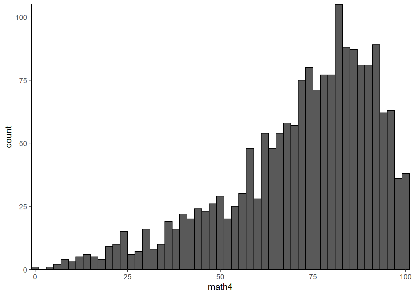
So, back to the original question; while the result is significant statistically, is it significant economically? Is it big? My impression from looking at these data is that no, it is not big. In this data, an extra $1,000 represents a relatively large budgetary increase that would have a very small impact on test scores. An extra $1,000 will not transform a poorly-performing school into a school with even middling math scores, nor will it transform an average-performing school into a top performer.
Perhaps this conclusion sits well with you. Perhaps it does not. Regardless, the correct path forward is not to condescendingly say “I told you so” with misplaced sense of smug sanctimoniousness to those who do not like this conclusion, or to go on social media to decry me as someone who hates education and eats children to try to get me canceled for wrongthink.
The correct path forward in either case is to ask the question as to whether or not this is the right model; has the analysis captured all of the relevant variables, or is something missing? One illustrates the accuracy of a model by demonstrating that it is specified correctly and nothing is missing, and one demonstrates the weakness of a model by arguing that something is wrong or missing, and showing that, if corrected, the coefficient I was interpreting changes in a meaningful way.
5.6 Wrapping Up
At this point, you should be able to use R to estimate a simple bivariate or multivariate OLS regression and to interpret the regression output. We will next turn to some of the key assumptions of regression analysis.
5.7 End of Chapter Exercises
Bivariate Regression: For items 1-3, you should a) create a scatterplot that includes a regression line, b) estimate the regression and display it using stargazer, c) identify the 3 largest outliers in the data (i.e. those with the largest residuals in absolute value terms), and d) interpret your findings from a-c.
wooldridge:winehas 3 interesting variables to use as dependent variables against wine consumption.In the
fivethirtyeight:pulitzerdata, can \(pctchg\_circ\) be explained by the Pulitzer prize winners at each newspaper?Look at the relationship between the the drop in output and the duration of strikes using the
AER:StrikeDurationdata.
Multivariate Regression:
Using
AER:CigarettesB, estimate a demand function for cigarettes. Use \(packs\) as your dependent variable. Does your demand curve slope downward? Are cigarettes a normal good? Since this is a log-log regression, the coefficient on price is the price elasticity of demand. Typically, we assume cigarettes are inelastic, is that what you are finding? What do you think might be going on here?Use the
AER:Electricity1955data to estimate a Cobb-Douglas cost function. Once you load the data, type?Electricity1955and use the code for Example 7.3 in the “Examples” section to estimate the model and test whether or not electricity has constant returns to scale.
Model Building: For each of the following, examine the data (and the help file for the data) to try and build a good multivariate regression. Think carefully about which variables to use as your dependent variable and as your independent variables.
AER:MASchoolshas 2 possible dependent variables to model as a function of school district attributes, \(score4\) and \(score8\).AER:CASchoolsis another interesting school dataset.Predict student grades using the
wooldridge:attenddata.