Chapter 1 Introductions are in Order
This chapter serves two general purporses. The first purpose is to introduce the concept of econometrics and answer such questions as:
- What is econometrics?
- Who uses econometrics?
- How does econometrics relate to other disciplines?
The second, and longer, focus of the chapter is to introduce the computer program R. This section is written with the assumption that this is the reader’s first foray into programming of any sort, so we will be starting with very basic questions:
- What are R and RStudio and how do you get them?
- How do I install this software?
- What kind of programs are they?
- How does one get help with R?
1.1 Introducing Econometrics
Econometrics is the branch of economics that applies statistics to economic theory. Thus, as statistics is a sub-iscipline of mathematics, some math is unavoidable when doing econometrics. However, the emphasis of this book is not econometric theory, it is applied econometrics. Thus, our focus will be more on the application and interpretation of econometrics than the mathematical underpinnings of the subject.
Less mathy does not necessarily mean easier. While the theoretical underpinning of econometrics is found in calculus, linear algebra, and probability theory, the application of econometrics requires at least an intuitive understanding of the math and a heavy dose of computer programming skills. In short, while this text will attempt to keep the use of calculus and linear algebra to a minimum, to actually do econometrics we are going to focus heavily on learning basic computer programming skills using the R language.
The fundamental building block of econometrics is ordinary least squares regression (OLS), which will be introduced in Chapter 5 and extended in chapters 6 and 7. OLS regression will create our basis for understanding to tackle more sophisticated methods, like probit/logit modeling in Chapter 8, time series in Chapter 10, and myriad other methods.
The fundamental methods of OLS, probit/logit, and time series are not only key tools in economics, but are key tools across a wide variety of disciplines throughout the social sciences, hard sciences, and quantitative areas of business. While people in these areas may be using these techniques for slightly different purposes, or may call them by different names, at the end of the day, developing an understanding these techniques provides you with a skillset that is useful in a wide variety of contexts well beyond academic economics.
Prior to tackling regression analysis, or indeed any of the other more sophisticated methods that build upon OLS, we will learn some R basics in Chapter 2 and how to use R to do some of the things it is already assumed you know how to do using other methods; for example, calculating descriptive statistics and making graphs (Chapter 3), and basic inferential statistics (e.g. hypothesis testing, ANOVA) in Chapter 4.
1.2 Introducing R
R is an open source programming/scripting language. It is broadly used in Econometrics, but has tons of other applications. It is a commonly used program in any academic discipline that relies upon statistical analysis, so researchers across the social (economics, sociology, psychology, etc) and physical sciences (epidemiology, biology, meteorology, etc) use R. Moreover, there is an increasing use of R for data visualization and analytics, so R is becoming widely used in the business world by people doing market analytics, business analytics, data mining, financial/data/research analysis, data journalism, actuarial science, and so forth. In short, the list is long. Moreover, while the focus of this text is on using R for econometrics, the fundamental methods of econometrics (particularly OLS, logit/probit, and time series) are the fundamental methods of nearly all fields utilizing R as well.
There are many other programs out there that are capable of the same types of data analysis and graphics as is R. That said, while R is not the only program of its kind, it is likely the the one used in the greatest variety of fields which lends to its usefulness. In the world of economics, the more commonly used software packages include SAS, SPSS, Stata, and to lesser extents programs like Eviews, Matlab, Python, and even Microsoft Excel.
Some Pros of R:
- price (free!)
- powerful and extensible
- purpose built for statistics
- probably here to stay
Some Cons of R:
- steep learning curve
- tough to keep track of extensions (packages)
- language and syntax can be inconsistent between packages
To begin, install 2 pieces of software: R and RStudio. R is the program that does the computation, while RStudio is an IDE (Integrated Development Environment), which is a fancy term for a program that makes programming a lot easier because it helps keep track of everything you are working on in one place. The good news is that they are both free and will work in Windows, Mac, or Linux environment. Make sure you install R before installing RStudio!
Go ahead and do it now; I’ll wait!

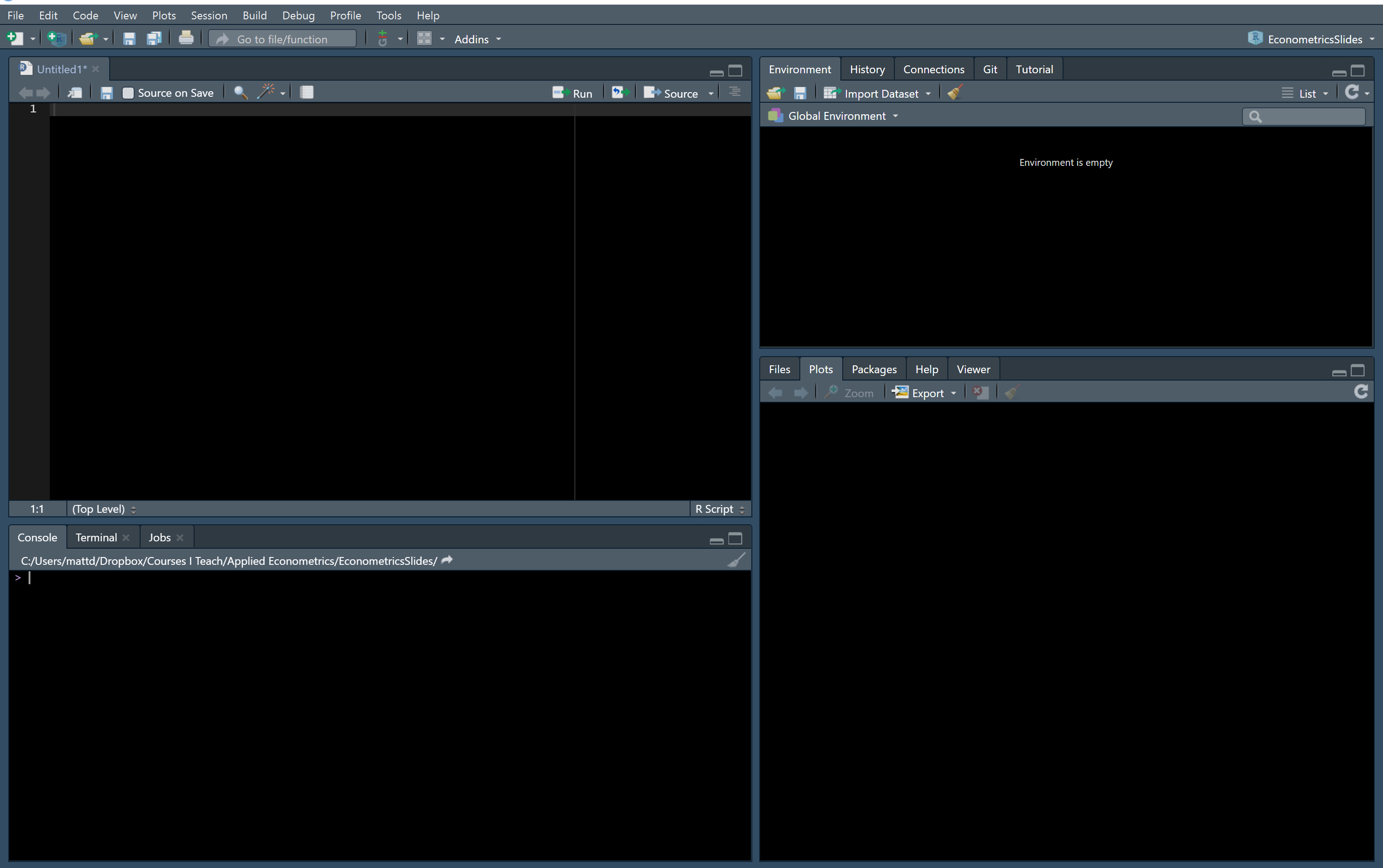
Let’s start with a brief overview of the RStudio environment. The basic layout of Rstudio has 4 panes:
Note that this looks a little different from what RStudio looks like “out of the box” but the differences are small.
The bottom left pane is the console window. R lives in the console window,and you can use R interactively here.
R is a command line interpreter that can be used either interactively or with scripts. Interactive use refers to a situation in which the user types a command into R and R immediately evaluates that command. A script is a set of commands that doesn’t get evaluated until the user tells it to. As an example of interactive use, if I type If I type 2+2 into the console window:
2+2## [1] 4R is certainly capable of being the world’s most elaborate calculator, and I am happy that I was not told that the answer is 5. But R is capable of much, much more than being a calculator.
For the most part, everything you do in R fits into one of three categories. You are either
- Creating objects (everything is an object),
- Performing functions on objects to create new objects, or
- Looking at objects
Typically, these tasks are done as part of a script, which brings us to the top left pane: the editor window. This is where you will spend most of your time writing. This panel is where you can write a script or examine the objects in your environment. A script is simply a set of commands that are fed into R sequentially to create output.
To see this in action, here is a short script that you can type into the editor pane that does something that you probably learned about in an introductory statistics course: a two-sample t-test:
data(mtcars)
mean(mtcars$mpg[mtcars$cyl==4])
mean(mtcars$mpg[mtcars$cyl==6])
test1 <- t.test(mtcars$mpg[mtcars$cyl==6], mtcars$mpg[mtcars$cyl==4])
pander::pander(test1, split.cells = c(1,1,50,1,1,1))
Before we talk about what each line does, let’s see the results of this script:
## [1] 26.66364## [1] 19.74286| Test statistic | df | P value | Alternative hypothesis | mean of x | mean of y |
|---|---|---|---|---|---|
| -4.719 | 12.96 | 0.0004048 * * * | two.sided | 19.74 | 26.66 |
Let’s look at this script, line-by-line, keeping the objects/functions framework in mind. The first line was:
data(mtcars) When R evaluates the first line, an object named mtcars is loaded into memory for us to play with. When you installed R, you installed a handful of datasets that R uses for documentation; mtcars is one of the many such datasets preloaded into R. The data in mtcars includes data from Motor Trend magazine in 1974 about car fuel consumption. The object mtcars is a specific type of object called a Data Frame, which is basically just a spreadsheet where the rows are the observations and the columns are the variables. Specifically, we will be looking at the variables relating to fuel efficiency (mpg) and engine size (cyl).
The next two lines were:
mean(mtcars$mpg[mtcars$cyl==4])
mean(mtcars$mpg[mtcars$cyl==6])
Because mtcars is a data frame, we can refer to the object as mtcars. We can also refer to columns within the object by using the dollar sign ($) and subsets of the data using [braces]. The first line, therefore, performs the function mean on the variable mpg in the data frame mtcars, but only for observations where the value of the variable cyl is equal to 4. Predictably, the second line does the exact same thing but for 6 cylinder automobiles.
When we evaluated this code, We saw that the mean of 4 cylinder cars was 26.6636364 and the mean of 6 cylinder cars was 19.7428571. A natural question to ask is whether or not this difference is statistically significant, which suggests that the right approach is to calculate a two-sample t-test, which is what line four does:
test1 <- t.test(mtcars$mpg[mtcars$cyl==6], mtcars$mpg[mtcars$cyl==4]) This line is easist read from right to left. This line uses another function, t.test, to calculate the two-sample t-test of whether or not the mpg of 6 cylinder cars is significantly different from the mpg of 4 cylinder cars. The little arrow <- assigns the results of the t-test to an object called test1, which will be an object type called a list.
The general syntax used is:
new object <- function with old object(s)
Like with the data frames above, you can refer to items (or sub-objects) within in this object with the $ as well. For example, one of the sub-objects within test1 is called conf.int, which is the confidence interval from my t-test. If I wanted utilize the confidence interval, I could could refer to test1\$conf.int.
It is notable that line 4 does the t-test, saves the results of the t-test as an object called test1, but it doesn’t actually tell us what the results are! To see the results, I could simply evaluate the line test1, but often you want your results to be nicely formatted, which is where line 5 comes in:
pander::pander(test1, split.cells = c(1,1,50,1,1,1)) This line uses a function called pander. The function pander is not part of r, rather, it is part of a package called pander, which had to be installed separately. The syntax here is package::function, so the expression pander::pander tells r to look in the package called pander for the function called pander, and pander is going to take the object test1 and make a pretty table from it. This all may seem a bit confusing at first, but don’t worry, we will discuss in more detail how packages work in Chapter 2.
Returning to our tour of RStudio, The top right pane is your environment Window. You can see what objects and variables are stored in memory. If you click on a data frame that is in your environment, you will be able to view that data as a spreadsheet in your editor window.
Finally, the bottom right pane has a bunch of different stuff. The most common and useful views down there are:
- Help
- Package info
- Plots/Graphs
- Directory structure
At this point, you may want to play around with some of the stuff found in the menu under Tools -> Global Options. You can change the way RStudio looks by editing the appearance. If you want a dark theme, make sure you change the theme to “Modern” or “Sky”. I would suggest choosing a theme that has a lot of contrasting colors to make reading your code easier. One of the primary benefits of using RStudio, especially when you are just learning, is the automatic color coding done by themes. I typically use Tomorrow Night Bright, but also like Cobalt, Merbivore Soft, and Vibrant Ink.
Another useful configuration to know about is under “Packages” – a CRAN mirror is where R gets packages from. CRAN mirrors are typically updated daily. RStudio defaults to using the CRAN mirror called “Global (CDN) - RStudio”. This is usually fine, and is run on the Amazon Cloud. If you have issues, though, you might choose a mirror that is close to you geographically to speed up your downloads.
There are a variety of ways to get help using R. Under Help -> Cheatsheets, RStudio has a bunch of coding cheatsheets that are super useful for when you are trying to figure out how to do things. You can find a more comprehensive list of cheatsheets at https://rstudio.com/resources/cheatsheets/. Cheatsheets may be worth printing out and keeping handy while working, especially while learning new packages.
More generally, if you need help in R there are tons of online sources. Beyond just googling things (which actually works most of the time), you can try:
- rseek.org is a search engine for R related issues.
- Online message boards (Reddit has /rstats, Stack Overflow has tons of R Q/A, community.rstudio.com, etc…)
- R ebooks are often free! Many of them are on RPubs.org
- YouTube has tons of videos on R.
- Twitter has a big R community – look for hashtags like #rstats, #tidytuesday, #rladies, #tidyverse, #rtweet