Chapter 8 Categorical Dependent Variables
Until now, we have been limited to using numeric variables as our dependent variables. In this chapter we look at how we can use OLS modeling for categorical dependent variables. We begin with the linear probability model and move on to the related but generally better logit and probit models. This set of models is designed for looking at dichotomous dependent variables – variables with only 2 possible outcomes. These types of outcomes are of the sort that can be answered as a yes or no type question, for example:
- Was a job candidate hired?
- Did a customer make a purchase?
- Was a patient cured?
- Did a product break?
- Did a politician vote for a specific bill?
As you might be starting to suspect, there are tons of interesting questions that can be answered with these types of models!
While not often utilized in economics, there are versions of probit and logit that are designed for multinomial (categorical variables with more than 2 outcomes) and ordered (multinomial variables whose levels can be ordered from worst to best, lowest to highest, etc.) dependent variables.
This chapter introduces a few packages that have not yet been used in this text. If they are not already installed on your computer, you may need to instell margins, jtools, mlogit, and/or MASS. Additionally, jtools requires a couple more packages to be installed to do what we will be asking it to do, broom and huxtable:
install.packages("margins")
install.packages("jtools")
install.packages("broom")
install.packages("huxtable")
install.packages("mlogit")
install.packages("MASS")
Finally, we load some datasets into memory, mostly from the AER, fivethirtyeight, MASS, and wooldridge packages.
data(k401ksubs)
data(SmokeBan)
data(affairs)
data(recid)
data(steak_survey)
data(comma_survey)
data(card)
data(CreditCard)
data(HMDA)
data(PSID1976)
data(ResumeNames)
data(card)
data(Titanic)
data(housing)
8.1 The Linear Probability Model
The linear probability model (LPM) is the easiest place to begin – while the model is generally thought to be inferior to probit or logit (for reasons that will be discussed in this section), estimating and interpreting the model is far more straightforward because it is literally just an OLS regression with a dummy variable as our dependent variable.
Let’s start with a simple bivariate model; it should help develop the intuition of predicting dichotomous outcomes without getting too complicated too quickly. We will use the k401ksubs dataset in the wooldridge package, which contains 9275 individual level observations. We will start by seeing whether or not income level, inc is predictive of whether or not an individual participates in a 401k account, captured in the p401k variable.
Let’s start by just putting the two variables we are going to analyze into a smaller dataframe called retdata and look at some summary statistics.
retdata <- k401ksubs %>%
    dplyr::select(inc, p401k) # Advisable to use dplyr::select because MASS has a select function that might override the one in dplyr.
summary(retdata)
## inc p401k
## Min. : 10.01 Min. :0.0000
## 1st Qu.: 21.66 1st Qu.:0.0000
## Median : 33.29 Median :0.0000
## Mean : 39.25 Mean :0.2762
## 3rd Qu.: 50.16 3rd Qu.:1.0000
## Max. :199.04 Max. :1.0000How do we interpret the results of the p401k variable? Because it is coded as a dummy variable, p401k=1 tells us that an individual has a 401k account, and p401k=0 tells us they do not. The mean of 0.2762264 tells us that 27.6% of the individuals in the data set have a 401k account.
If the question we seek to ask is whether or not higher income levels are predictive of 401k participation, we might think to see if there is a different mean income of the two groups:
k401ksubs %>% group_by(p401k) %>%
    summarize(mean = mean(inc))
## # A tibble: 2 x 2
## p401k mean
## <int> <dbl>
## 1 0 35.2
## 2 1 49.8As a reminder, we could have gotten the same summary statistics using mean(retdata$inc[retdata$p401k == 0]) and mean(retdata$inc[retdata$p401k == 1]).
These results do suggest that individuals who participate in their company’s 401k program tend to have higher incomes on average. The next step is to determine whether or not we can establish that this relationship is statistically significant.
In the methods we’ve seen thus far, e.g. dummy variables as in Chapter 7, the categorical variable has been the independent variable, whereas here, the categorical variable is the dependent variable. In other words, what we have learned so far is how to use a categorical variable as a predictor, now we will be learning how to actually predict a categorical variable.
The linear probability model is simple to estimate; we run a regression using p401k as our dependent variable with inc as the sole independent variable.
Luckily, the k401ksubs data has coded the p401k variable as a dummy for us already; if it were not and instead was coded as a factor, we would need an extra step (e.g. we could create a dummy variable using the ifelse() command, we could use the as.numeric() command, etc.). We will see examples of this sort later!
reg1a <- lm(p401k ~ inc, data = k401ksubs)
stargazer(reg1a, type = "text")
##
## ===============================================
## Dependent variable:
## ---------------------------
## p401k
## -----------------------------------------------
## inc 0.005***
## (0.0002)
##
## Constant 0.079***
## (0.009)
##
## -----------------------------------------------
## Observations 9,275
## R2 0.073
## Adjusted R2 0.073
## Residual Std. Error 0.430 (df = 9273)
## F Statistic 734.022*** (df = 1; 9273)
## ===============================================
## Note: *p<0.1; **p<0.05; ***p<0.01What does this result tell us? The \(\hat{\beta} = .005\) tells us that, for every $1,000 increase in income, the expected probability of an individual participating in the 401k program increases by half a percentage point.
\[\begin{equation} Probability\:of\:401k\:Participation_{i} = .079 + .005 \cdot income_i \end{equation}\]
Just as with a regression, we can calculate a predicted probability by plugging in values for \(income_i\); for example, we would estimate that somebody with $50,000 income (\(inc_i=50\)), as:
\[\begin{equation} Probability\:of\:401k\:Participation_{i} = .079 + .005 \cdot 50 = 32.9\% \end{equation}\]
What if we wanted to predict the probability of 401k participation for somebody with an income of $190,000 (\(inc_i=190\))
\[\begin{equation} Probability\:of\:401k\:Participation_{i} = .079 + .005 \cdot 190 = 102.9\% \end{equation}\]
Somehow the model gives this individual a greater than 100% chance of participating in their company’s 401k program! This is a problem, especially considering that \(inc_i=190\) isn’t extrapolation. The first major issue with using the Linear Probability Model is that it is often possible for a predicted value to negative or greater than 100%.
In the graph below, we can see that there are quite a few datapoints to the right of where the blue prediction line crosses 1:
k401ksubs %>% ggplot(aes(x = inc, y = p401k)) +
    geom_point() +
    geom_smooth(method = lm, se = FALSE) +
    theme_classic()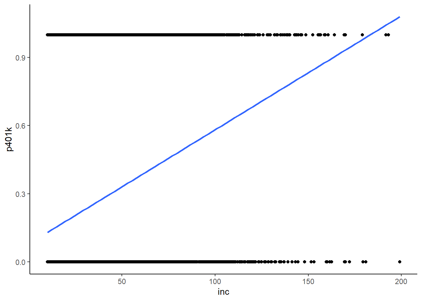
A second problem with the LPM becomes apparent when examining the Q-Q plot. Recall, the Q-Q plot examines the residuals of the model, and the Q-Q plot is expected to be a relatively straight line. For a the linear probability model, it will almost certainly never be so:
qqnorm(reg1a$residuals)
qqline(reg1a$residuals)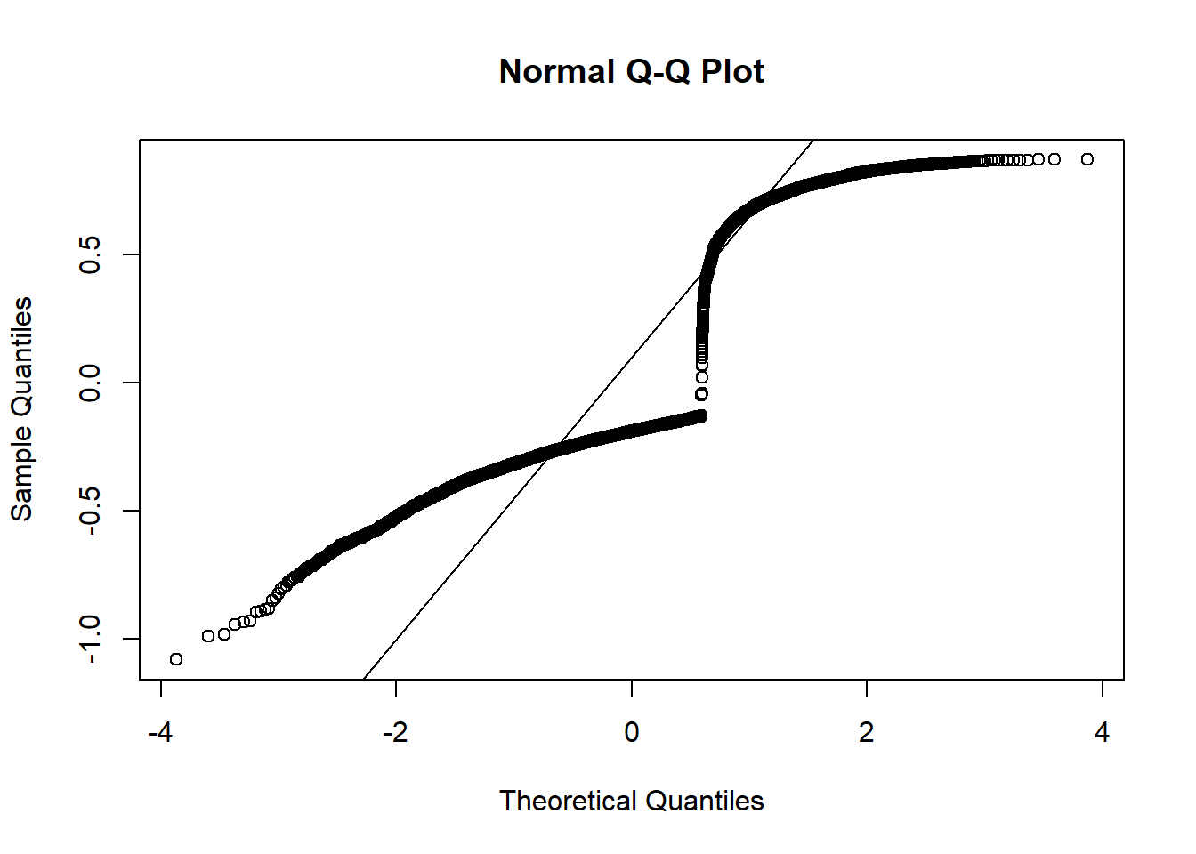
This is a funky looking graph, but this level of heteroskedasticity is completely expected for a linear probability model; you are predicting a probability, so most of your predictions are between 0 and 1. However, the outcome variable p401k can ONLY be 0 or 1. This pretty much guarantees that you will have too many huge outliers.
8.2 Probit and Logit
For these two reasons, the linear probability model is rarely used. Instead, we turn to estimating a logit or probit model, either of which mitigates both of these problems.

Estimating these models are fairly straightforward and require the glm() command; GLM stands for Generalized Linear Model. Let’s estimate both the logit and probit models:
reg1b <- glm(p401k ~ inc, family = binomial(link = "logit"), data = k401ksubs)
reg1c <- glm(p401k ~ inc, family = binomial(link = "probit"), data = k401ksubs)
The syntax for these are very similar to the syntax for lm; the function is specified in the same way (p401k ~ inc), the data is specified in the same way (data = k401ksubs), the only difference is that you need to specify the family option.
While estimating the model is fairly straightforward, interpreting the results is not. Let’s look at the 3 results, side-by-side:
stargazer(reg1a, reg1b, reg1c, type = "text")##
## ===================================================================
## Dependent variable:
## -----------------------------------------------
## p401k
## OLS logistic probit
## (1) (2) (3)
## -------------------------------------------------------------------
## inc 0.005*** 0.024*** 0.015***
## (0.0002) (0.001) (0.001)
##
## Constant 0.079*** -1.966*** -1.197***
## (0.009) (0.049) (0.028)
##
## -------------------------------------------------------------------
## Observations 9,275 9,275 9,275
## R2 0.073
## Adjusted R2 0.073
## Log Likelihood -5,144.242 -5,139.835
## Akaike Inf. Crit. 10,292.480 10,283.670
## Residual Std. Error 0.430 (df = 9273)
## F Statistic 734.022*** (df = 1; 9273)
## ===================================================================
## Note: *p<0.1; **p<0.05; ***p<0.01Some things stand out. First, probit and logit do not have an \(R^2\), instead, they have goodness of fit measures called log-likelihood and AIC. Next, the estimated \(\hat{\alpha}\) and \(\hat{beta}\) look very different from those of the linear model. Interpreting \(\hat{\alpha}\) and \(\hat{beta}\) in this form is quite difficult; it requires wrapping ones mind around the concept of log-likelihood and odds ratios and other such things. If you are just interested in predictive modeling, these results are sufficient. But for the sake of learning how to interpret the model, we will learn how to convert these coefficients to a format that is interpreted like OLS coefficients shortly.
First though, let’s look at a graph of what we just estimated.
k401ksubs %>% ggplot(aes(x = inc, y = p401k)) +
    geom_point() +
    geom_smooth(method = lm, color = "cornflowerblue", se = FALSE) +
    stat_smooth(method = "glm",
                method.args = list(family = binomial(link = "probit")),
                color = "mediumorchid",
                se = FALSE) +
    stat_smooth(method = "glm",
                method.args = list(family = binomial(link = "logit")),
                color = "limegreen",
                se = FALSE) +
    theme_classic()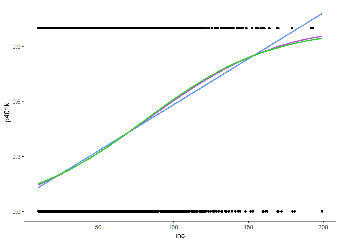
The blue line is the linear model that we plotted earlier, the red and green lines are the probit and logit models, respectively. Two points of note:
- The probit and logit models are very similar to each other. Logit used to be far more popular than probit 30+ years ago, because logit requires significantly less computing power than probit, but those concerns are no longer relevant given the state of modern computing. Logit is often preferred in disciplines like biostats, because the logit coefficients have a useful interpretation in terms of odds ratios. Generally speaking, there may be a slight preference for probit in economics, but for the most part, it doesn’t much matter which one you use. I personally prefer probit, but if somebody wants to collaborate on a paper and they estimate a logit I’m not gonna worry about it.

- The probit and logit models are clearly non-linear, and they will asymptotically approach 0 and 1 but will never actually hit 0 or 1.
The fact that the model is non-linear provides a useful place to think about the concept of the margin. In economics, the idea of “marginal” is very similar to the idea of “additional”; for example, the marginal cost of production is the additional cost incurred from producing one more item, marginal utility is the additional utility received from consuming a tiny bit more of something, and so on. With that in mind, the estimated values of \(\hat{\beta}\) from an OLS regression have a very similar interpretation – a small, one unit change in your \(X\) variable leads to a \(\hat{\beta}\) sized increase in your \(Y\) variable. In the linear model, the value of \(\hat{\beta}\) is constant; that is, regardless of the value of \(X\), the marginal effect of \(X\) on \(Y\) is the same: \(\hat{\beta}\). In a non-linear model like probit or logit, the marginal effect of \(X\) on \(Y\) varies by the value of \(X\); where the curve is relatively flat, the marginal effect of \(X\) on \(Y\) is relatively small, whereas when the curve is relatively steep, the marginal effect of \(X\) on \(Y\) is relatively large.
The upshot of all of this is that it will take some work to be able to interpret our probit and logit estimates in the same way we interpret our OLS estimates. To do so, we need to obtain marginal effects from our probit and logit model. Luckily, there are multiple packages we can install that will do all the work for us. We will use the margins package.
There are two primary methods of calculating marginal effects:
- Marginal Effect at the Means (MEM) – find the mean of all of your independent variables, and calculate the marginal effect of each variable at that point.
- Average Marginal Effect (AME) – find the marginal effect for every observation in the data, and calculate the mean of those marginal effects.
MEM is easier to calculate, though in my opinion AME is the more generally appropriate method. By default, margins uses the AME option. The syntax for the margins() function is quite simple – simply feed it a logit or probit object.
Unfortunately, stargazer does not work well with the output of the margins command, so we will switch to use export_summs() from the jtools package.
reg1bmargins <- margins(reg1b)
reg1cmargins <- margins(reg1c)
export_summs(reg1a, reg1bmargins, reg1cmargins)| Model 1 | Model 2 | Model 3 | |
|---|---|---|---|
| (Intercept) | 0.08 *** | ||
| (0.01) | |||
| inc | 0.01 *** | 0.00 *** | 0.00 *** |
| (0.00) | (0.00) | (0.00) | |
| N | 9275 | 0 | 0 |
| R2 | 0.07 | ||
| *** p < 0.001; ** p < 0.01; * p < 0.05. | |||
As you can see from the above output, export_summs() does something very similar to stargazer, but one drawback of export_summs() is that you usually have to doctor the results a bit more to make it readable. For example, the statistical significance stars don’t match those of stargazer (and therefore are not those standard in economics), though this can be manually changed by adding a stars option. Another issue is that it does not identify the number of observations in the model correctly. Finally, I will also add a couple options to aid with readability: naming the models, adding AIC (more on this shortly), getting rid of the observation count, and changing the number format to add a couple of decimal places so we aren’t looking at a table full of zeroes. With probit and logit it is very useful to know how to use the number_format option, since the phenomenon we are measuring is a probability.
huxtable::set_width(export_summs(reg1a, reg1bmargins, reg1cmargins,
                                 number_format = "%.4f",
                                 stars = c(`***` = 0.01, `**` = 0.05, `*` = 0.1),
                                 statistics = c(N = NULL, "AIC"),
                                 model.names = c("OLS", "Logit", "Probit")),
.8)| OLS | Logit | Probit | |
|---|---|---|---|
| (Intercept) | 0.0789 *** | ||
| (0.0085) | |||
| inc | 0.0050 *** | 0.0045 *** | 0.0046 *** |
| (0.0002) | (0.0002) | (0.0002) | |
| AIC | 10689.7415 | 10292.4841 | 10283.6707 |
| *** p < 0.01; ** p < 0.05; * p < 0.1. | |||
Here we see that the estimated marginal effects of the logit and probit model are actually very similar to each other. This shouldn’t be a huge surprise; remember the curves above looked really similar to each other as well.
It is also of note that there is no intercept term reported for the logit or probit; this is expected because it is impossible to have a marginal change in the constant! The estimated marginal effects are also a bit smaller than the OLS estimates – but are they more accurate?
With OLS, we usually use \(R^2\) to compare models, but probit and logit do not have an \(R^2\) so we need to find a measure that allows us to compare between model types. This is where the AIC comes in: the Akiake Information Criterion (AIC) provides us with a way to compare probits/logits to OLS. I have included in the table above, but they are also obtainable with the AIC() command. For AIC, lower scores are better. A good rule of thumb for information criteria is that a difference of 10 is a big difference.
AIC(reg1a)## [1] 10689.74AIC(reg1b)## [1] 10292.48AIC(reg1c)## [1] 10283.67The probit and logit have very similar values for AIC, with probit being a bit better in this case, and they are both significantly lower than that of the regression model, indicating that either model is far better than the OLS estimates.
8.3 More Examples Using Probit and Logit
As the probit and logit models are a) generally a better fit than the linear probability model, and b) mostly a matter of preference, the rest of this chapter will example exclusively probit models. If you feel that logit is more your jam, go ahead and do some logits instead. But remember, friends don’t let friends estimate Linear Probability Models.
As with OLS regressions, we can include multiple independent variables (though it’s usually not a good idea to include interaction effects), non-linear terms, dummy variables, and so forth. Let’s estimate a probit with the same 401k data as above, adding a quadratic term for income and \(pira\), a dummy variable that is equal to 1 if the individual has an IRA:
\[\begin{equation} Probability\:of\:401k\:Participation_{i} = \alpha + \beta_1 \cdot income_i + \beta_2 \cdot income_i^2 + \beta_3 \cdot pira_i \end{equation}\]
The following code will estimate this regression and display it with the probit from up above:
reg1d <- glm(p401k ~ inc + I(inc^2) + pira, data = k401ksubs, family = binomial(link = "probit"))
reg1dmargins <- margins(reg1d)
huxtable::set_width(export_summs(reg1cmargins, reg1dmargins,
                                 number_format = "%.4f",
                                 statistics = c(N = NULL, "AIC", "BIC"),
                                 stars = c(`***` = 0.01, `**` = 0.05, `*` = 0.1)),
.6)| Model 1 | Model 2 | |
|---|---|---|
| inc | 0.0046 *** | 0.0057 *** |
| (0.0002) | (0.0002) | |
| pira | 0.0515 *** | |
| (0.0104) | ||
| AIC | 10283.6707 | 10144.7679 |
| BIC | 10297.9409 | 10173.3082 |
| *** p < 0.01; ** p < 0.05; * p < 0.1. | ||
The estimated \(\hat{\beta}=0.0515\) on the \(pira\) dummy variable is relatively straightforward to interpret; all else equal, the probability than an individual with a value of \(pira=1\) has a 401k is 5.15 percentage points higher than an individaual with a value of \(pira=0\).
The presentation of the income variable may be a bit of a surprise, however; wasn’t there a squared term in the original model? If we look at the original regression results (i.e. before we transformed them into marginal effects), we can see that the model was indeed estimated with a squared term!
huxtable::set_width(export_summs(reg1d,
                                number_format = "%.4f",
                                stars = c(`***` = 0.01, `**` = 0.05, `*` = 0.1)),
.4)| Model 1 | |
|---|---|
| (Intercept) | -1.5894 *** |
| (0.0473) | |
| inc | 0.0309 *** |
| (0.0018) | |
| I(inc^2) | -0.0001 *** |
| (0.0000) | |
| pira | 0.1669 *** |
| (0.0338) | |
| N | 9275 |
| AIC | 10144.7679 |
| BIC | 10173.3082 |
| Pseudo R2 | 0.1188 |
| *** p < 0.01; ** p < 0.05; * p < 0.1. | |
Not only was it there, but it was significantly less than zero, suggesting diminishing returns to income! So where did the squared term go in the report from the margins() command? Because we specified the model using the I() function, R knew that the \(inc\) and \(inc^2\) terms in the model are the same variable, so the margins() command knows to combine the two when calculating the marginal effect. This is a useful benefit of using the I() function to specify non-linearities rather than just creating variables and putting them in the model.
Let’s turn to a different data set, SmokeBan in the AER package. We will use a probit model to predict whether or not one is a smoker based on their age, gender, race, education, and whether or not there is a workplace smoking ban.
As before, the scripting workflow here is to:
store the results of a
glm()in an object;run that regression object through the
margins()function, and save that as an object;display the object created by
margins()withexport_summs().
reg2a <- glm(smoker ~ ban + age + education + afam + hispanic + gender, data = SmokeBan, family = binomial(link = "probit"))
reg2amargins <- margins(reg2a)
huxtable::set_width(export_summs(reg2amargins,
                                 number_format = "%.4f",
                                 stars = c(`***` = 0.01, `**` = 0.05, `*` = 0.1)),
.4)| Model 1 | |
|---|---|
| afamyes | -0.0231 |
| (0.0149) | |
| age | -0.0012 *** |
| (0.0003) | |
| banyes | -0.0455 *** |
| (0.0088) | |
| educationcollege | -0.2687 *** |
| (0.0190) | |
| educationhs | -0.0892 *** |
| (0.0191) | |
| educationmaster | -0.3104 *** |
| (0.0195) | |
| educationsome college | -0.1564 *** |
| (0.0191) | |
| genderfemale | -0.0329 *** |
| (0.0086) | |
| hispanicyes | -0.0897 *** |
| (0.0116) | |
| nobs | 0 |
| null.deviance | 11074.3324 |
| df.null | 9999.0000 |
| logLik | -5252.3489 |
| AIC | 10524.6977 |
| BIC | 10596.8012 |
| deviance | 10504.6977 |
| df.residual | 9990.0000 |
| nobs.1 | 10000.0000 |
| *** p < 0.01; ** p < 0.05; * p < 0.1. | |
This is another model in which there are a considerable number of dummy explanatory variables; as with OLS, we interpret them with respect to the omitted group. For example, \(\hat{\beta}=-0.0329\) for the female dummy indicates that females are 3.3 percentage points less likely to smoke than males. It seems that the strongest predictor of smoking is education; we can see the simple percentages in graphic form with a stacked bar chart:
SmokeBan %>% ggplot(aes(fill = smoker, x = education)) +
    geom_bar(position = "fill") +
    theme_classic()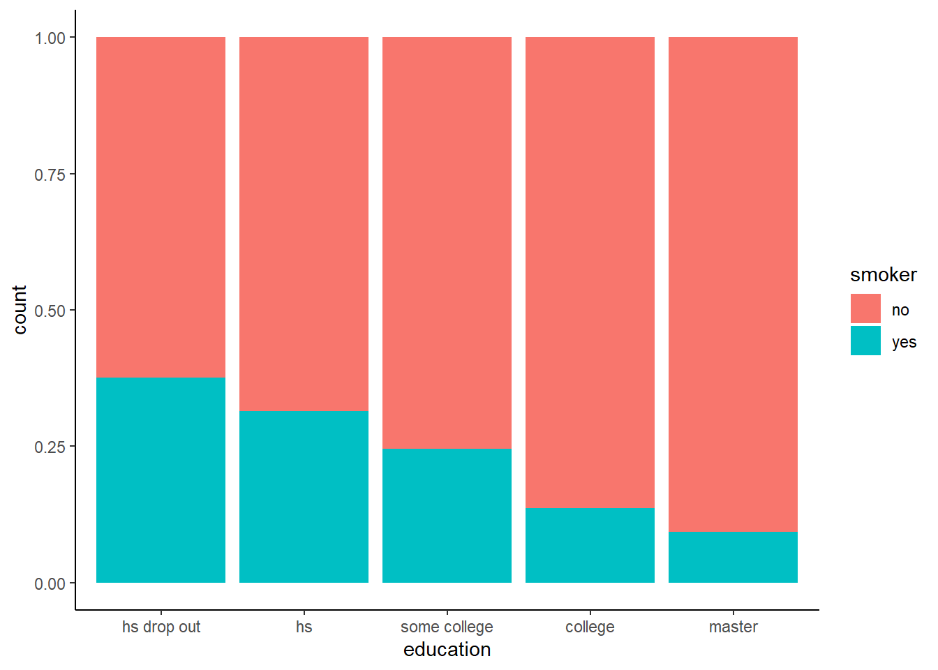
The above graph looks at the raw data in the original SmokeBan dataset. However, now that we have estimated this probit model, we could similarly plot the predicted values of whether or not someone smokes by calculating the mean of the fitted values by each educational group:
smokepred <- SmokeBan
smokepred$fitted <- reg2a$fitted.values
smokepred %>% ggplot(aes(y = fitted, x = education)) +
    geom_bar(stat = "summary", fun.fill = "mean", fill = "orangered3") +
    theme_classic()
## Warning: Ignoring unknown parameters: fun.fill## No summary function supplied, defaulting to `mean_se()`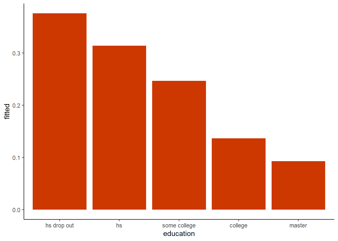
We can also compare the proportions from the raw data with the conditional probabilities from the probit, as below. They are fairly close, but not the same, because the fitted values are taking into account all of the independent variables from the probit model!
smokepred %>%
  group_by(education) %>%
  summarize(raw = mean(as.numeric(smoker)-1), conditional = mean(fitted))
## # A tibble: 5 x 3
## education raw conditional
## <fct> <dbl> <dbl>
## 1 hs drop out 0.376 0.376
## 2 hs 0.314 0.314
## 3 some college 0.246 0.246
## 4 college 0.136 0.136
## 5 master 0.0926 0.0927Do smoking bans reduce smoking? The estimated coefficient on smoking bans \(\hat{\beta}=-0.0455\) suggests that perhaps they do, though there may be questions of reverse causation here; perhaps non-smokers are more willing to work at non-smoking workplaces than are smokers.
Let’s take another look at the affairs dataset. We predict whether or not an individual had an estramarital affair with gender, whether or not they have kids, education level, length of marriage, measures of religiosity, and their rating of their marital happiness.
reg3a <- glm(affair ~ male + yrsmarr + kids + relig + educ + ratemarr, data = affairs, family = binomial(link = "probit"))
reg3amargins <- margins(reg3a)
huxtable::set_width(export_summs(reg3amargins,
                                 number_format = "%.4f",
                                 stars = c(`***` = 0.01, `**` = 0.05, `*` = 0.1)),
                    .4)
## Warning in nobs.default(m, use.fallback = TRUE): no 'nobs' method is available| Model 1 | |
|---|---|
| educ | 0.0032 |
| (0.0076) | |
| kids | 0.0662 |
| (0.0469) | |
| male | 0.0347 |
| (0.0365) | |
| ratemarr | -0.0772 *** |
| (0.0144) | |
| relig | -0.0544 *** |
| (0.0145) | |
| yrsmarr | 0.0065 * |
| (0.0037) | |
| nobs | 0 |
| null.deviance | 675.3770 |
| df.null | 600.0000 |
| logLik | -308.0657 |
| AIC | 630.1314 |
| BIC | 660.9216 |
| deviance | 616.1314 |
| df.residual | 594.0000 |
| nobs.1 | 601.0000 |
| *** p < 0.01; ** p < 0.05; * p < 0.1. | |
As one might expect, happily married and highly religious individuals are less likely to have an affair than otherwise. If we look more deeply at the data descriptions with data(affairs), we see that the religiosity and marital happiness variables are coded as such:
relig: 5 = very relig., 4 = somewhat, 3 = slightly, 2 = not at all, 1 = anti
ratemarr: 5 = vry hap marr, 4 = hap than avg, 3 = avg, 2 = smewht unhap, 1 = vry unhap
As these are coded as numbers, running the probit model with the variables as-is implies that the variables are somehow measures; our closer look, however, suggests that this data is actually ordinal, and therefore are factors, not numeric. As such, it may make sense to ask R to treat these variables like factor variables instead of numbers, which we will do with the as.numeric() function.
reg3b <- glm(affair ~ male + yrsmarr + kids + as.factor(relig) + educ + as.factor(ratemarr), data = affairs, family = binomial(link = "probit"))
reg3bmargins <- margins(reg3b)
huxtable::set_width(export_summs(reg3amargins, reg3bmargins,
                                 number_format = "%.4f",
                                 stars = c(`***` = 0.01, `**` = 0.05, `*` = 0.1),
                                 model.names = c("Measured", "Factors")),
.6)| Measured | Factors | |
|---|---|---|
| educ | 0.0032 | 0.0030 |
| (0.0076) | (0.0075) | |
| kids | 0.0662 | 0.0589 |
| (0.0469) | (0.0469) | |
| male | 0.0347 | 0.0362 |
| (0.0365) | (0.0364) | |
| ratemarr | -0.0772 *** | |
| (0.0144) | ||
| relig | -0.0544 *** | |
| (0.0145) | ||
| yrsmarr | 0.0065 * | 0.0066 * |
| (0.0037) | (0.0037) | |
| ratemarr2 | 0.0075 | |
| (0.1348) | ||
| ratemarr3 | -0.1744 | |
| (0.1300) | ||
| ratemarr4 | -0.2290 * | |
| (0.1259) | ||
| ratemarr5 | -0.2970 ** | |
| (0.1257) | ||
| relig2 | -0.1983 *** | |
| (0.0759) | ||
| relig3 | -0.1238 | |
| (0.0792) | ||
| relig4 | -0.2779 *** | |
| (0.0734) | ||
| relig5 | -0.2718 *** | |
| (0.0814) | ||
| nobs | 0 | 0 |
| null.deviance | 675.3770 | 675.3770 |
| df.null | 600.0000 | 600.0000 |
| logLik | -308.0657 | -302.7147 |
| AIC | 630.1314 | 631.4294 |
| BIC | 660.9216 | 688.6111 |
| deviance | 616.1314 | 605.4294 |
| df.residual | 594.0000 | 588.0000 |
| nobs.1 | 601.0000 | 601.0000 |
| *** p < 0.01; ** p < 0.05; * p < 0.1. | ||
Above, the two models are displayed side-by-side. If we inspect the \(\hat{\beta}\) coefficients on both the religiosity and marriage happiness variables, we see that there may be a little more nuance revealed when treating them with the as.factor() command than simply treating them like measured variables. For example, there does not seem to be a difference between \(relig = 4\) and \(relig = 5\), nor does there appear to be a difference between \(ratemarr = 1\) and \(ratemarr = 2\), and \(relig = 3\) seems to be worse for affairs than \(relig = 2\). So which model is better? Sorting this question out is a good place to use the information criteria.
They have similar measures of AIC, but the Bayesian Information Criterion (BIC) is actually better for the model on the left by a pretty big margin: 660.921587 - 688.611143 = -27.689556 is considerably more than a difference of 10. The AIC and BIC work a lot like Adjusted \(R^2\) in regression in that they “penalize” you for having more independent variables than you need to model the data. In this context, it means that even though the model on the right explains more of the variation in the dependent variable, it does so using a lot more information, and the information isn’t adding enough to the predictive power of the model to justify its inclusion.
Let’s work through one more probit example to see how we can estimate marginal effects for specific values of our independent variables. This is especially important for calculating the marginal effects of interaction effects, which is super tricky in these models.
Let’s use the recid data in the wooldridge package. This data looks at prison recidivism, and the variable cens indicates whether or not an individual released from prison wound up back in prison (\(cens = 0\)) or did not (\(cens = 1\)) at some point in the next 6-7 years. Let’s suppose we believe that recidivism is influenced by whether or not an individual was in the North Carolina prison work program, and that we suspect the effectiveness of the prison work program is somehow affected by years of education. We will model \(cens\) as a function the interaction between the prisoner’s years of education and whether or not the participated in the North Carolina prison work program and other control variables.
reg4a <- glm(cens ~ educ*workprg + age +I(age^2) + drugs + alcohol + black + tserved,
             data = recid,
             family = binomial(link = "probit"))
huxtable::set_width(export_summs(reg4a), .4)| Model 1 | |
|---|---|
| (Intercept) | -0.57 |
| (0.36) | |
| educ | -0.00 |
| (0.02) | |
| workprg | -0.51 |
| (0.29) | |
| age | 0.01 *** |
| (0.00) | |
| I(age^2) | -0.00 ** |
| (0.00) | |
| drugs | -0.26 ** |
| (0.08) | |
| alcohol | -0.43 *** |
| (0.09) | |
| black | -0.36 *** |
| (0.07) | |
| tserved | -0.01 *** |
| (0.00) | |
| educ:workprg | 0.04 |
| (0.03) | |
| N | 1445 |
| AIC | 1833.72 |
| BIC | 1886.47 |
| Pseudo R2 | 0.10 |
| *** p < 0.001; ** p < 0.01; * p < 0.05. | |
We see that all of our control variables are significant, but none of our variables of interest are. Next, let’s run the regression object through the margins() function to see some easier-to-interpet results:
reg4amargins <- margins(reg4a)
huxtable::set_width(export_summs(reg4amargins,
                                 number_format = "%.4f",
                                 stars = c(`***` = 0.01, `**` = 0.05, `*` = 0.1)),
.4)| Model 1 | |
|---|---|
| age | 0.0010 *** |
| (0.0002) | |
| alcohol | -0.1550 *** |
| (0.0312) | |
| black | -0.1303 *** |
| (0.0248) | |
| drugs | -0.0916 *** |
| (0.0289) | |
| educ | 0.0072 |
| (0.0054) | |
| tserved | -0.0038 *** |
| (0.0006) | |
| workprg | -0.0302 |
| (0.0267) | |
| nobs | 0 |
| null.deviance | 1921.9600 |
| df.null | 1444.0000 |
| logLik | -906.8582 |
| AIC | 1833.7163 |
| BIC | 1886.4750 |
| deviance | 1813.7163 |
| df.residual | 1435.0000 |
| nobs.1 | 1445.0000 |
| *** p < 0.01; ** p < 0.05; * p < 0.1. | |
Of note is that both the quadratic term on \(age\) and the interaction effect are not presented here; again, this is to be expected because of the way that marginal effects are calculated.
Finally, to test our hypothesis that there is an interaction between the work program and education, we will use the at option in margins(). Let’s look at the marginal effects for \(educ = 8\), \(educ = 12\), and \(educ = 16\):
reg4amargins0 <- margins(reg4a, at = list(educ = 8))
reg4amargins1 <- margins(reg4a, at = list(educ = 12))
reg4amargins2 <- margins(reg4a, at = list(educ = 16))
export_summs(reg4amargins, reg4amargins0, reg4amargins1, reg4amargins2,
             number_format = "%.3f",
             stars = c(`***` = 0.01, `**` = 0.05, `*` = 0.1),
model.names = c("AME", "Education = 8", "Education = 12", "Education = 16"))| AME | Education = 8 | Education = 12 | Education = 16 | |
|---|---|---|---|---|
| age | 0.001 *** | 0.001 *** | 0.001 *** | 0.001 *** |
| (0.000) | (0.000) | (0.000) | (0.000) | |
| alcohol | -0.155 *** | -0.156 *** | -0.153 *** | -0.148 *** |
| (0.031) | (0.032) | (0.031) | (0.030) | |
| black | -0.130 *** | -0.131 *** | -0.129 *** | -0.124 *** |
| (0.025) | (0.025) | (0.024) | (0.024) | |
| drugs | -0.092 *** | -0.092 *** | -0.090 *** | -0.087 *** |
| (0.029) | (0.029) | (0.029) | (0.028) | |
| educ | 0.007 | 0.007 | 0.007 | 0.006 |
| (0.005) | (0.006) | (0.005) | (0.005) | |
| tserved | -0.004 *** | -0.004 *** | -0.004 *** | -0.004 *** |
| (0.001) | (0.001) | (0.001) | (0.001) | |
| workprg | -0.030 | -0.057 * | 0.006 | 0.065 |
| (0.027) | (0.032) | (0.035) | (0.066) | |
| nobs | 0 | 0 | 0 | 0 |
| null.deviance | 1921.960 | 1921.960 | 1921.960 | 1921.960 |
| df.null | 1444.000 | 1444.000 | 1444.000 | 1444.000 |
| logLik | -906.858 | -906.858 | -906.858 | -906.858 |
| AIC | 1833.716 | 1833.716 | 1833.716 | 1833.716 |
| BIC | 1886.475 | 1886.475 | 1886.475 | 1886.475 |
| deviance | 1813.716 | 1813.716 | 1813.716 | 1813.716 |
| df.residual | 1435.000 | 1435.000 | 1435.000 | 1435.000 |
| nobs.1 | 1445.000 | 1445.000 | 1445.000 | 1445.000 |
| *** p < 0.01; ** p < 0.05; * p < 0.1. | ||||
Because these are all margins calculated on the same model, the model parameters (i.e. the stuff below the coefficients: n, AIC, etc) are the same for each column. As we can see, estimating the marginal effect at differing levels of education reveals that the North Carolina prison work program seems to have a negative and significant effect on individuals with low levels of education. It might also be instructive to estimate the marginal effects for \(workprg = 0\) and \(workprg = 1\):
reg4amarginsnowork <- margins(reg4a, at = list(workprg = 0))
reg4amarginswork <- margins(reg4a, at = list(workprg = 1))
huxtable::set_width(export_summs(reg4amargins,
                                 reg4amarginsnowork,
                                 reg4amarginswork,
                                 number_format = "%.4f",
                                 stars = c(`***` = 0.01, `**` = 0.05, `*` = 0.1),
                                 model.names = c("AME", "No Work Program", "Work Program")),
.8)| AME | No Work Program | Work Program | |
|---|---|---|---|
| age | 0.0010 *** | 0.0010 *** | 0.0010 *** |
| (0.0002) | (0.0002) | (0.0002) | |
| alcohol | -0.1550 *** | -0.1533 *** | -0.1567 *** |
| (0.0312) | (0.0307) | (0.0318) | |
| black | -0.1303 *** | -0.1289 *** | -0.1318 *** |
| (0.0248) | (0.0246) | (0.0252) | |
| drugs | -0.0916 *** | -0.0906 *** | -0.0926 *** |
| (0.0289) | (0.0286) | (0.0293) | |
| educ | 0.0072 | -0.0001 | 0.0157 ** |
| (0.0054) | (0.0075) | (0.0074) | |
| tserved | -0.0038 *** | -0.0038 *** | -0.0039 *** |
| (0.0006) | (0.0006) | (0.0006) | |
| workprg | -0.0302 | -0.0291 | -0.0312 |
| (0.0267) | (0.0261) | (0.0273) | |
| nobs | 0 | 0 | 0 |
| null.deviance | 1921.9600 | 1921.9600 | 1921.9600 |
| df.null | 1444.0000 | 1444.0000 | 1444.0000 |
| logLik | -906.8582 | -906.8582 | -906.8582 |
| AIC | 1833.7163 | 1833.7163 | 1833.7163 |
| BIC | 1886.4750 | 1886.4750 | 1886.4750 |
| deviance | 1813.7163 | 1813.7163 | 1813.7163 |
| df.residual | 1435.0000 | 1435.0000 | 1435.0000 |
| nobs.1 | 1445.0000 | 1445.0000 | 1445.0000 |
| *** p < 0.01; ** p < 0.05; * p < 0.1. | |||
Looked at this way, we can see that education is not a good predictor of recidivism for individuals not in the work program, but it is for individuals in the work program.
8.4 Ordered and Multinomial Probit
If our dependent variable has more than 2 possible levels, then we need to use slightly the more advanced methods of Ordered Probit and/or Multinomial Probit. If the levels of our dependent variable are ordered, we use ordered probit, and if they are unordered, we use multinomial probit. Generally speaking, these two models are far more advanced than the probit models we saw above, so we will only briefly look at these models.
Some applications of ordered probit might include:
Your dependent variable is a Likert scale (e.g. the responses are strongly disagree, disagree, …, strongly agree).
You are modeling purchase decisions on a scale (e.g. does a visitor to Disney World stay at a value resort, moderate resort, or luxury resort?).
Sometimes all you have is ordered data even if numeric data in principal exists, such as education level, income level, etc.
By contrast, mulntinomial probit would be called for in situations where the response variable doesn’t have a natural ordering:
You are modeling an unordered purchase decision, such as whether or not somebody purchased a Xbox Series X, PS5, or Nintendo Switch.
You are modeling individual preferences (e.g. you survey people and ask them their favorite fast food restaurant).
Let’s work through one example of an ordered probit. A warning: interpreting the coefficients on these models is very tricky; we will focus on interpreting signs and significance, but interpreting magnitudes will be left as an advanced exercise for the interested reader.
The command for an ordered probit, polr(), is part of the MASS package, so if you haven’t run install.packages("MASS") and/or library(MASS), now is the time. We will make use of the housing dataset contained within the MASS package.
head(housing)## Sat Infl Type Cont Freq
## 1 Low Low Tower Low 21
## 2 Medium Low Tower Low 21
## 3 High Low Tower Low 28
## 4 Low Medium Tower Low 34
## 5 Medium Medium Tower Low 22
## 6 High Medium Tower Low 36The variable \(Sat\) measures housing satisfaction on an ordered scale, so an ordered probit model is appropriate here. Note that the unusual coding of the data requires us to use the weights = Freq option.
reg5a <- polr(Sat ~ Infl + Type + Cont, weights = Freq, data = housing, method = "probit")
summary(reg5a)
## Call:
## polr(formula = Sat ~ Infl + Type + Cont, data = housing, weights = Freq,
## method = "probit")
##
## Coefficients:
## Value Std. Error t value
## InflMedium 0.3464 0.06414 5.401
## InflHigh 0.7829 0.07643 10.244
## TypeApartment -0.3475 0.07229 -4.807
## TypeAtrium -0.2179 0.09477 -2.299
## TypeTerrace -0.6642 0.09180 -7.235
## ContHigh 0.2224 0.05812 3.826
##
## Intercepts:
## Value Std. Error t value
## Low|Medium -0.2998 0.0762 -3.9371
## Medium|High 0.4267 0.0764 5.5850
##
## Residual Deviance: 3479.689
## AIC: 3495.689Essentially, the ordered probit model estimates the probability of each of the possible outcome values at the same time, and assigns a probability to each outcome. Because the order of the dependent variable is from worst appraisal of housing satisfaction (\(Sat = Low\)) to the highest appraisal (\(Sat = High\)), we interpret negative coefficients as reducing somebody’s appraisal of their housing satisfaction. Since these independent variables are dummies, we interpret them as before, with reference to the omitted variable. Finally, while there are no stars displayed here, we can use t-values to get the same information about significance. A good rule of thumb is that a t-value greater than 2 (or less than -2) indicates a statistically significant coefficient.
This model generates multiple predicted probabilities – one for each of the possible values of the dependent variable. Here, the ordered probit generates 3 such probabilities. The predicted value for an observation, then, is the outcome with the highest probability of occurring. We can take a look at the predicted values for each observation with the following code:
temphousing <- predict(reg5a, housing, type = "probs")
temphousing <- as.data.frame(temphousing)
temphousing <- temphousing %>%
    bind_cols(housing) %>%
    filter(Sat == "Low") %>%
    select(- c(Sat,Freq))
tibble(temphousing)
## # A tibble: 24 x 6
## Low Medium High Infl Type Cont
## <dbl> <dbl> <dbl> <fct> <fct> <fct>
## 1 0.382 0.283 0.335 Low Tower Low
## 2 0.259 0.273 0.468 Medium Tower Low
## 3 0.139 0.221 0.639 High Tower Low
## 4 0.519 0.262 0.219 Low Apartment Low
## 5 0.383 0.283 0.334 Medium Apartment Low
## 6 0.231 0.265 0.503 High Apartment Low
## 7 0.467 0.273 0.260 Low Atrium Low
## 8 0.334 0.283 0.383 Medium Atrium Low
## 9 0.194 0.251 0.555 High Atrium Low
## 10 0.642 0.220 0.138 Low Terrace Low
## # ... with 14 more rows
## # i Use `print(n = ...)` to see more rows8.5 Wrapping Up
Probit and logit models are a essential addition to our econometric skill set as they allow us to extend our data skills into explaining categorical phenonema. We have also looked briefly at the ordinal and multinomial versions of probit and logit; while the programming skills requried for these models is a bit beyond the scope of this text, I hope that you can see their potential usefulness.
Next, we turn to models for censored and count variables.
8.6 End of Chapter Exercises
Probit and Logit:
Model Building: For each of the following, examine the data (and the help file for the data) to try and build a good multivariate probit/logit model. Think carefully about the variables you have to choose among to explain your dependent variable with. Consider strongly the use of non-linear or interaction effects in your model. Finally, interpret your results with the help of margins and export_summs to make your results more interpretable.
AER:CreditCard- model \(card\), a binary variable denoting whether or not a credit card application was accepted.AER:HMDA- model \(deny\), looking in particular for discrimination against black borrowers (the \(afam\) dummy). Does discrimination go away when controlling for all relevant factors?AER:PSID1976- model \(participation\) as a function of education, age, number of children, family income, etc.AER:ResumeNames- model \(call\), looking in particular for discrimination against individuals with “black names.” This type of analysis is called an “audit study”wooldridge:card- model \(enroll\), a binary measuring whether or not a student enrolled at a college.datasets:Titanic- model \(Survived\), and see if “women and children first” was really a thing! To convert thisTitanicinto something usable by theglm()function, use the following code first:
data(Titanic)
tempdata <- as.data.frame(Titanic)
titaniclong <- tempdata[rep(1:nrow(tempdata), tempdata$Freq), -5]
Ordinal Models:
Same model building instructions as above. These can be tricky because the data needs some formatting before usage.
The
fivethirtyeightdatasetsteak_surveyhas an interesting ordinal variable, \(steak\_prep\), which comes from a survey of how well done Americans like their steak.The
comma_surveyin thefivethirtyeightdataset includes a variable called \(care\_proper\_grammar\) that is a likert scale on how much people care about proper use of grammar.In the
wooldridge:happinessdataset, thehappyvariable is ordinal.