Chapter 7 Categorical Independent Variables
Thus far, we have only considered models in which the independent variables are numeric. Now, we expand our understanding of OLS regression to include categorical independent variables as well. This notebook will discuss the use of dummy (indicator) variables and interaction effects in regression modelling.
Let’s begin by loading in the data that will used in this chapter from the AER and wooldridge packages:
data(CPS1985)
data(HousePrices)
data(diamonds)
data(gpa2)
data(TeachingRatings)
data(CPS1988)
data(GrowthDJ)
data(CollegeDistance)
data(happiness)
data(beauty)
data(campus)
data(twoyear)
7.1 Dummy Variables
Categorical independent variables are incorporated into a regression model via dummy variables. A dummy variable is simply a variable that takes on a value of 1 if an observation is of a specific category, and 0 otherwise. For example, let’s consider the CPS1985 data:
head(CPS1985)## wage education experience age ethnicity region gender occupation
## 1 5.10 8 21 35 hispanic other female worker
## 1100 4.95 9 42 57 cauc other female worker
## 2 6.67 12 1 19 cauc other male worker
## 3 4.00 12 4 22 cauc other male worker
## 4 7.50 12 17 35 cauc other male worker
## 5 13.07 13 9 28 cauc other male worker
## sector union married
## 1 manufacturing no yes
## 1100 manufacturing no yes
## 2 manufacturing no no
## 3 other no no
## 4 other no yes
## 5 other yes noOne of the variables in this data set, gender, is categorical and has two possible values (levels) in the data: male or female.
summary(CPS1985$gender)## male female
## 289 245We can see that R considers this to be a factor variable:
class(CPS1985$gender)## [1] "factor"Let’s transform this into a set of dummy variables. Because our factor variable has 2 possible levels, we can make 2 different dummy variables out of it: a male dummy and a female dummy.
tempdata <- CPS1985
tempdata$female <- ifelse(tempdata$gender == "female", 1, 0)
tempdata$male <- ifelse(tempdata$gender == "male", 1, 0)
Let’s verify that the dummies look right:
tempdata[168:177, c(7, 12, 13)]## gender female male
## 167 male 0 1
## 168 male 0 1
## 169 female 1 0
## 170 female 1 0
## 171 male 0 1
## 172 female 1 0
## 173 female 1 0
## 174 male 0 1
## 175 male 0 1
## 176 female 1 0What if we wanted to look at a categorical variable with more than 2 levels, like occupation?
summary(CPS1985$occupation)## worker technical services office sales management
## 156 105 83 97 38 55This factor variable has 6 levels, so you would create 6 dummies. Luckily, in R you do not need to create dummy variables; if you run a regression with a factor variable it will do all of this in the background. However, we will use these created dummies a few times in this chapter to see the intuition of what is going on here, and in the real world, often data is already coded in dummy format so it is useful to understand how it works.
As an additional note, if a categorical variable has \(L\) levels, you would only need \(L-1\) dummy variables. We will discuss why as we go along, but the reason lies in the multicollinearity assumption we saw in Chapter 6.
7.2 Anything ANOVA Does, Regression Does Better
In some circles, those are fighting words!
In Chapter 4, we looked at some methods of inferential statistics with categorical independent variables, particularly the 2-sample t-test and ANOVA. Recall, the two-sample t-test is when you have a numeric dependent variable that you think varies based on the value of a categorical independent variable that has two possible levels. An ANOVA is the same thing, but for categorical independent variables with 2 or more levels or multiple categorical variables.
Let’s use these two techniques to look at the wage gap in the CPS1985 data:
t.test(wage ~ gender, data = CPS1985)##
## Welch Two Sample t-test
##
## data: wage by gender
## t = 4.8853, df = 530.55, p-value = 1.369e-06
## alternative hypothesis: true difference in means between group male and group female is not equal to 0
## 95 percent confidence interval:
## 1.265164 2.966949
## sample estimates:
## mean in group male mean in group female
## 9.994913 7.878857summary(aov(wage ~ gender, data = CPS1985))## Df Sum Sq Mean Sq F value Pr(>F)
## gender 1 594 593.7 23.43 1.7e-06 ***
## Residuals 532 13483 25.3
## ---
## Signif. codes: 0 '***' 0.001 '**' 0.01 '*' 0.05 '.' 0.1 ' ' 1Fun aside: there is a variant of the ANOVA called the Welch One-Way Test that actually gets the same results as a 2-sample t-test:
oneway.test(wage ~ gender, data = CPS1985)##
## One-way analysis of means (not assuming equal variances)
##
## data: wage and gender
## F = 23.866, num df = 1.00, denom df = 530.55, p-value = 1.369e-06They mey look slightly different, because the t-test relies on the t-distribution and the one-way test relies on the F-distribution, except the F-distribution is just the t-distribution squared and the p-values are the same so really it is just the same thing. But I digress…
…But I guess if we are talking about how two different looking things are in fact the same thing, we should talk about ANOVA and Regression with dummy variables. We can use regression to obtain the exact same results as we did with the ANOVA above:
\[\begin{equation} Wage_{i} = \alpha + \beta female_i \end{equation}\]
reg1a <- lm(wage ~ female, data = tempdata)
stargazer(reg1a, type = "text")##
## ===============================================
## Dependent variable:
## ---------------------------
## wage
## -----------------------------------------------
## female -2.116***
## (0.437)
##
## Constant 9.995***
## (0.296)
##
## -----------------------------------------------
## Observations 534
## R2 0.042
## Adjusted R2 0.040
## Residual Std. Error 5.034 (df = 532)
## F Statistic 23.426*** (df = 1; 532)
## ===============================================
## Note: *p<0.1; **p<0.05; ***p<0.01It may be presented slighly differently, but this result is in fact identical to the ANOVA we saw before.
##              Df Sum Sq Mean Sq F value  Pr(>F)
## gender        1    594   593.7   23.43 1.7e-06 ***
## Residuals   532  13483    25.3
## ---
## Signif. codes: 0 '***' 0.001 '**' 0.01 '*' 0.05 '.' 0.1 ' ' 1The F-value is identical, and if you examine the ANOVA table from the regression model, you see even more identical looking stuff. The only difference is rounding:
## Analysis of Variance Table
##
## Response: wage
##            Df  Sum Sq Mean Sq F value    Pr(>F)
## female      1   593.7  593.71  23.426 1.703e-06 ***
## Residuals 532 13483.0   25.34
## ---
## Signif. codes:  0 '***' 0.001 '**' 0.01 '*' 0.05 '.' 0.1 ' ' 1
So with that aside out of the way, let’s return to the actual regression results:
stargazer(reg1a, type = "text")##
## ===============================================
## Dependent variable:
## ---------------------------
## wage
## -----------------------------------------------
## female -2.116***
## (0.437)
##
## Constant 9.995***
## (0.296)
##
## -----------------------------------------------
## Observations 534
## R2 0.042
## Adjusted R2 0.040
## Residual Std. Error 5.034 (df = 532)
## F Statistic 23.426*** (df = 1; 532)
## ===============================================
## Note: *p<0.1; **p<0.05; ***p<0.01What do these estimated coefficients mean? First, two definitions. The included group is a group that we have created a dummy variable for and included in the model. In this regression female is the included group. The omitted group is the group for which there is no dummy in the model. Here, male is the omitted group. For any categorical variable, you must have precisely one omitted group, for reasons that should become clear shortly.
The constant term is the average of the omitted group: the average male wage is $9.995. The \(\hat{\beta}\) on female is the difference between females and males. This result tells us that on average, females earn $2.116 less than males in the data, and that this difference in wages is statistically significant.
We can visualize this result with a boxplot:
tempdata %>% ggplot(aes(fill = gender, y = wage)) +
    geom_boxplot() +
    scale_fill_brewer(palette="Accent")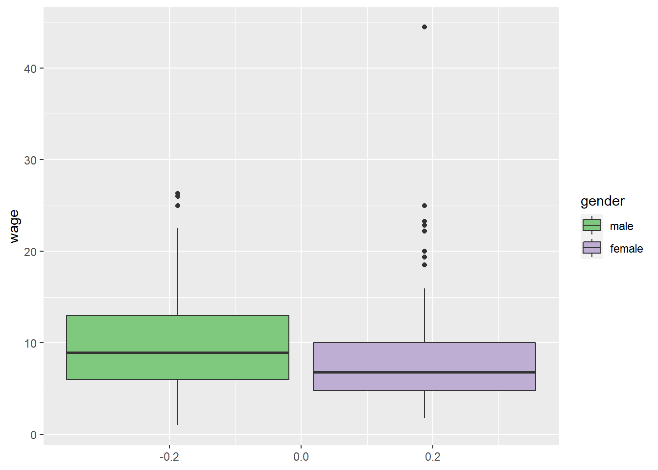
The regression results are telling us that the differences between these groups is in fact significant.
The regression results stored in the object reg1a were obtained using the dummy variables we created above. We don’t actually need to create dummy variables if the data are stored as factors. Estimating a regression using the factor variable gender gives the same results.
reg1b <- lm(wage ~ gender, data = tempdata)
stargazer(reg1a, reg1b, type = "text")
##
## ===========================================================
## Dependent variable:
## ----------------------------
## wage
## (1) (2)
## -----------------------------------------------------------
## female -2.116***
## (0.437)
##
## genderfemale -2.116***
## (0.437)
##
## Constant 9.995*** 9.995***
## (0.296) (0.296)
##
## -----------------------------------------------------------
## Observations 534 534
## R2 0.042 0.042
## Adjusted R2 0.040 0.040
## Residual Std. Error (df = 532) 5.034 5.034
## F Statistic (df = 1; 532) 23.426*** 23.426***
## ===========================================================
## Note: *p<0.1; **p<0.05; ***p<0.01What would have happened if we estimated a regression with the male dummies instead?
reg1c <- lm(wage ~ male, data = tempdata)
stargazer(reg1a, reg1c, type = "text")
##
## ===========================================================
## Dependent variable:
## ----------------------------
## wage
## (1) (2)
## -----------------------------------------------------------
## female -2.116***
## (0.437)
##
## male 2.116***
## (0.437)
##
## Constant 9.995*** 7.879***
## (0.296) (0.322)
##
## -----------------------------------------------------------
## Observations 534 534
## R2 0.042 0.042
## Adjusted R2 0.040 0.040
## Residual Std. Error (df = 532) 5.034 5.034
## F Statistic (df = 1; 532) 23.426*** 23.426***
## ===========================================================
## Note: *p<0.1; **p<0.05; ***p<0.01As before, the constant tells us the mean of the omitted group (female), and the \(\hat{\beta}\) on male is the difference between males and females. It should not be a surprise that it is simply the negative inverse of the female dummy from reg1a!
If you wanted to generate analogous results using female as the omitted group while using the factor variable gender, it’s fairly simple using the relevel() function:
reg1d <- lm(wage ~ relevel(gender, "female"), data = tempdata)
stargazer(reg1c, reg1d, type = "text")
##
## ===========================================================
## Dependent variable:
## ----------------------------
## wage
## (1) (2)
## -----------------------------------------------------------
## male 2.116***
## (0.437)
##
## relevel(gender, "female")male 2.116***
## (0.437)
##
## Constant 7.879*** 7.879***
## (0.322) (0.322)
##
## -----------------------------------------------------------
## Observations 534 534
## R2 0.042 0.042
## Adjusted R2 0.040 0.040
## Residual Std. Error (df = 532) 5.034 5.034
## F Statistic (df = 1; 532) 23.426*** 23.426***
## ===========================================================
## Note: *p<0.1; **p<0.05; ***p<0.01Thus far, we have excluded either the male or the female dummy. Why not simply estimate a regression with both dummies in it?
reg1e <- lm(wage ~ male + female, data = tempdata)
stargazer(reg1e, type = "text")
##
## ===============================================
## Dependent variable:
## ---------------------------
## wage
## -----------------------------------------------
## male 2.116***
## (0.437)
##
## female
##
##
## Constant 7.879***
## (0.322)
##
## -----------------------------------------------
## Observations 534
## R2 0.042
## Adjusted R2 0.040
## Residual Std. Error 5.034 (df = 532)
## F Statistic 23.426*** (df = 1; 532)
## ===============================================
## Note: *p<0.1; **p<0.05; ***p<0.01R won’t allow it, but why not? Recall the discussion from Chapter 6 regarding multicollinearity; we cannot have a variable that is a linear combination of other variables. This is often refered to as the dummy variable trap.

What would happen if you added the male dummy to the female dummy?
tempdata$tempvar <- tempdata$male + tempdata$female
tempdata[168:177, c(7, 12, 13, 14)]
## gender female male tempvar
## 167 male 0 1 1
## 168 male 0 1 1
## 169 female 1 0 1
## 170 female 1 0 1
## 171 male 0 1 1
## 172 female 1 0 1
## 173 female 1 0 1
## 174 male 0 1 1
## 175 male 0 1 1
## 176 female 1 0 1It seems that you will get a column of 1s, and a column of 1s will be collinear with the variable that is added to the regression to calculate the constant term. If you really wanted, you could run this regression with no constant term:
reg1f <- lm(wage ~ female + male - 1, data = tempdata)
stargazer(reg1f, type = "text")
##
## ===============================================
## Dependent variable:
## ---------------------------
## wage
## -----------------------------------------------
## female 7.879***
## (0.322)
##
## male 9.995***
## (0.296)
##
## -----------------------------------------------
## Observations 534
## R2 0.766
## Adjusted R2 0.765
## Residual Std. Error 5.034 (df = 532)
## F Statistic 869.622*** (df = 2; 532)
## ===============================================
## Note: *p<0.1; **p<0.05; ***p<0.01But there is really no point in doing so. You don’t get any added information, and if your research question is about the difference between the male and female groups, this regression doesn’t tell you that. You know that \(\hat{\beta_1} =7.879\) and \(\hat{\beta_2}=9.995\) are significantly different from zero, but you don’t know if the difference between \(\hat{\beta_1}\) and \(\hat{\beta_2}\) is significantly different, which is what you are trying to figure out!
In this data, gender is a factor variable with 2 levels–what if we have a factor with more than 2 levels, say occupation? We can call a regression model in much the same way:
reg2a <- lm(wage ~ occupation, data = tempdata)
stargazer(reg2a, type = "text")
##
## ================================================
## Dependent variable:
## ---------------------------
## wage
## ------------------------------------------------
## occupationtechnical 3.521***
## (0.590)
##
## occupationservices -1.889***
## (0.635)
##
## occupationoffice -1.004*
## (0.604)
##
## occupationsales -0.834
## (0.846)
##
## occupationmanagement 4.278***
## (0.733)
##
## Constant 8.426***
## (0.374)
##
## ------------------------------------------------
## Observations 534
## R2 0.180
## Adjusted R2 0.173
## Residual Std. Error 4.675 (df = 528)
## F Statistic 23.224*** (df = 5; 528)
## ================================================
## Note: *p<0.1; **p<0.05; ***p<0.01Here, constant is the average wage for the omitted group (worker), and the \(\hat{\beta}\) estimates for the various occupations are interpreted relative to the omitted group; for example, people whose occupation is “management” make on average $4.28 more than those whose occupation is “worker”, and that difference is statistically significant. While mathematically it does not matter which occupation is the omitted group, when doing hypothesis testing it is often most useful to omit the group with either the highest or lowest average.
reg2b <- lm(wage ~ relevel(occupation, "services"), data = tempdata)
stargazer(reg2b, type = "text")
##
## =====================================================================
## Dependent variable:
## ---------------------------
## wage
## ---------------------------------------------------------------------
## relevel(occupation, "services")worker 1.889***
## (0.635)
##
## relevel(occupation, "services")technical 5.410***
## (0.687)
##
## relevel(occupation, "services")office 0.885
## (0.699)
##
## relevel(occupation, "services")sales 1.055
## (0.916)
##
## relevel(occupation, "services")management 6.167***
## (0.813)
##
## Constant 6.537***
## (0.513)
##
## ---------------------------------------------------------------------
## Observations 534
## R2 0.180
## Adjusted R2 0.173
## Residual Std. Error 4.675 (df = 528)
## F Statistic 23.224*** (df = 5; 528)
## =====================================================================
## Note: *p<0.1; **p<0.05; ***p<0.01The releveled variables are a bit ugly in the table; this is because we releveled the factor variable inside the lm() command. We could also permanently relevel the variable with the relevel command and get cleaner looking regression tables:
tempdata$occupation <- relevel(tempdata$occupation, "services")
reg2c <- lm(wage ~ occupation, data = tempdata)
stargazer(reg2c, type = "text")
##
## ================================================
## Dependent variable:
## ---------------------------
## wage
## ------------------------------------------------
## occupationworker 1.889***
## (0.635)
##
## occupationtechnical 5.410***
## (0.687)
##
## occupationoffice 0.885
## (0.699)
##
## occupationsales 1.055
## (0.916)
##
## occupationmanagement 6.167***
## (0.813)
##
## Constant 6.537***
## (0.513)
##
## ------------------------------------------------
## Observations 534
## R2 0.180
## Adjusted R2 0.173
## Residual Std. Error 4.675 (df = 528)
## F Statistic 23.224*** (df = 5; 528)
## ================================================
## Note: *p<0.1; **p<0.05; ***p<0.01Just like with ANOVA, we can look at interaction effects with categorical variables as well. Let’s look at a wage regression with gender interacted with married. For comparison, these results are presented alongside regressions with just gender, just married, and both married and gender but not interacted.
The syntax is the same as before:
reg3aa <- lm(wage ~ gender, data = tempdata)
reg3ab <- lm(wage ~ married, data = tempdata)
reg3ac <- lm(wage ~ gender + married, data = tempdata)
reg3ad <- lm(wage ~ gender*married, data = tempdata)
stargazer(reg3aa, reg3ab, reg3ac, reg3ad, type = "text")
##
## =====================================================================================================================
## Dependent variable:
## ---------------------------------------------------------------------------------------------
## wage
## (1) (2) (3) (4)
## ---------------------------------------------------------------------------------------------------------------------
## genderfemale -2.116*** -2.128*** -0.095
## (0.437) (0.435) (0.735)
##
## marriedyes 1.087** 1.112** 2.521***
## (0.466) (0.456) (0.612)
##
## genderfemale:marriedyes -3.097***
## (0.907)
##
## Constant 9.995*** 8.312*** 9.272*** 8.355***
## (0.296) (0.377) (0.418) (0.494)
##
## ---------------------------------------------------------------------------------------------------------------------
## Observations 534 534 534 534
## R2 0.042 0.010 0.053 0.073
## Adjusted R2 0.040 0.008 0.049 0.068
## Residual Std. Error 5.034 (df = 532) 5.118 (df = 532) 5.011 (df = 531) 4.962 (df = 530)
## F Statistic 23.426*** (df = 1; 532) 5.437** (df = 1; 532) 14.789*** (df = 2; 531) 13.941*** (df = 3; 530)
## =====================================================================================================================
## Note: *p<0.1; **p<0.05; ***p<0.01Let’s focus on column 4, the model with interaction effects. This result is a bit trickier to interpret than a simple dummy variable, so let’s start with examining the regression model being estimated:
\[\begin{equation} Wage_i = \alpha + \beta_1 female_i +\beta_2 married_i +\beta_3 (female_i \: and \: married_i) \end{equation}\]
Essentially, we have 4 groups
- married female
- unmarried female
- married male
- unmarried male
For each group, the values of the dummies would look like:
| category | female | married | married and female |
| unmarried male | 0 | 0 | 0 |
| married male | 0 | 1 | 0 |
| unmarried female | 1 | 0 | 0 |
| married female | 1 | 1 | 1 |
In this model, the omitted group would be the group of individuals who have a 0 for each of the values of \(X\), so unmarried males are the omitted group, and the constant is their mean. To make predictions, you simply add in the value of \(\beta\) for any of the categories a particular individual belongs to. So how do we interpret the estimated coefficients?
stargazer(reg3ad, type = "text")##
## ===================================================
## Dependent variable:
## ---------------------------
## wage
## ---------------------------------------------------
## genderfemale -0.095
## (0.735)
##
## marriedyes 2.521***
## (0.612)
##
## genderfemale:marriedyes -3.097***
## (0.907)
##
## Constant 8.355***
## (0.494)
##
## ---------------------------------------------------
## Observations 534
## R2 0.073
## Adjusted R2 0.068
## Residual Std. Error 4.962 (df = 530)
## F Statistic 13.941*** (df = 3; 530)
## ===================================================
## Note: *p<0.1; **p<0.05; ***p<0.01The ones on gender and marital status are fairly straightforward; they state that women make on average 9 cents less than men (this result is not statistically significant), and that married people make on average $2.52 more than unmarried people (this result is statistically significant). Interpreting the interaction term is a bit trickier, and how you do it depends on your hypothesis. To illustrate this idea, the following two statements are both supported by the regression (and are actually saying the same thing!):
- The effect of gender on wages is $3.10 larger for married women than it is for single women.
- The effect of being married on wages is $3.10 bigger for men than it is for women.
All of the results so far are identical to those we could have obtained using ANOVA; so why is regression superior to ANOVA? Because ANOVA can only handle categorical independent variables, but regression can easily incorporate both categorical and numerical variables into the same model!
7.3 Combining Numeric and Categorical Independent Variables
Let’s continue with the CPS1985 data and consider the following model:
\[\begin{equation} Wage_i = \alpha + \beta_1 education_i +\beta_2 female_i \end{equation}\]
Education is a numeric variable while female is categorical. The resulting regression looks like:
reg4a <- lm(wage ~ education + gender, data = CPS1985)
stargazer(reg4a, type = "text")
##
## ===============================================
## Dependent variable:
## ---------------------------
## wage
## -----------------------------------------------
## education 0.751***
## (0.077)
##
## genderfemale -2.124***
## (0.403)
##
## Constant 0.218
## (1.036)
##
## -----------------------------------------------
## Observations 534
## R2 0.188
## Adjusted R2 0.185
## Residual Std. Error 4.639 (df = 531)
## F Statistic 61.616*** (df = 2; 531)
## ===============================================
## Note: *p<0.1; **p<0.05; ***p<0.01In this model, \(\hat{\beta_1}=0.751\) tells us that an additional year of education is correlated with an increase in wages of $0.75 per hour. This point estimate does not vary between genders. The estimated \(\hat{\beta_2} = -2.124\) suggests that, for a given amount of education, females are predicted to earn $2.12 less than a male. Essentially, this model is estimating 2 regression lines, one for males and another for females, but both lines have the same slope.
Let’s do a little algebra to see how this works. Inserting the estimated coefficients from the regression into the regression equation yields:
\[\begin{equation} Wage_i = 0.22 + 0.75 \cdot education_i - 2.12 \cdot female_i \end{equation}\]
The \(female\) variable is a dummy, and takes on a value of 1 if the observation is female and 0 otherwise. So this means that, for males, the regression equation is:
\[\begin{equation} Wage_i = 0.22 + 0.75 \cdot education_i - 2.12 \cdot 0 Wage_i = 0.22 + 0.75 \cdot education_i \end{equation}\]
While for females the equation is
\[\begin{equation} Wage_i = 0.22 + 0.75 \cdot education_i - 2.12 \cdot 1 Wage_i = 0.22 + 0.75 \cdot education_i - 2.12 Wage_i = -1.90 + 0.75 \cdot education_i \end{equation}\]
Graphically, therefore, this model looks like:
CPS1985 %>% ggplot(aes(x = education, y = wage, color = gender)) +
    geom_point() +
    scale_color_manual(values = c("cornflowerblue","indianred")) +
    geom_abline(slope = .751, intercept = .218, color = "darkblue", size = 1.2) +
    geom_abline(slope = .751, intercept = .218-2.124, color = "firebrick4", size = 1.2) +
    theme_classic()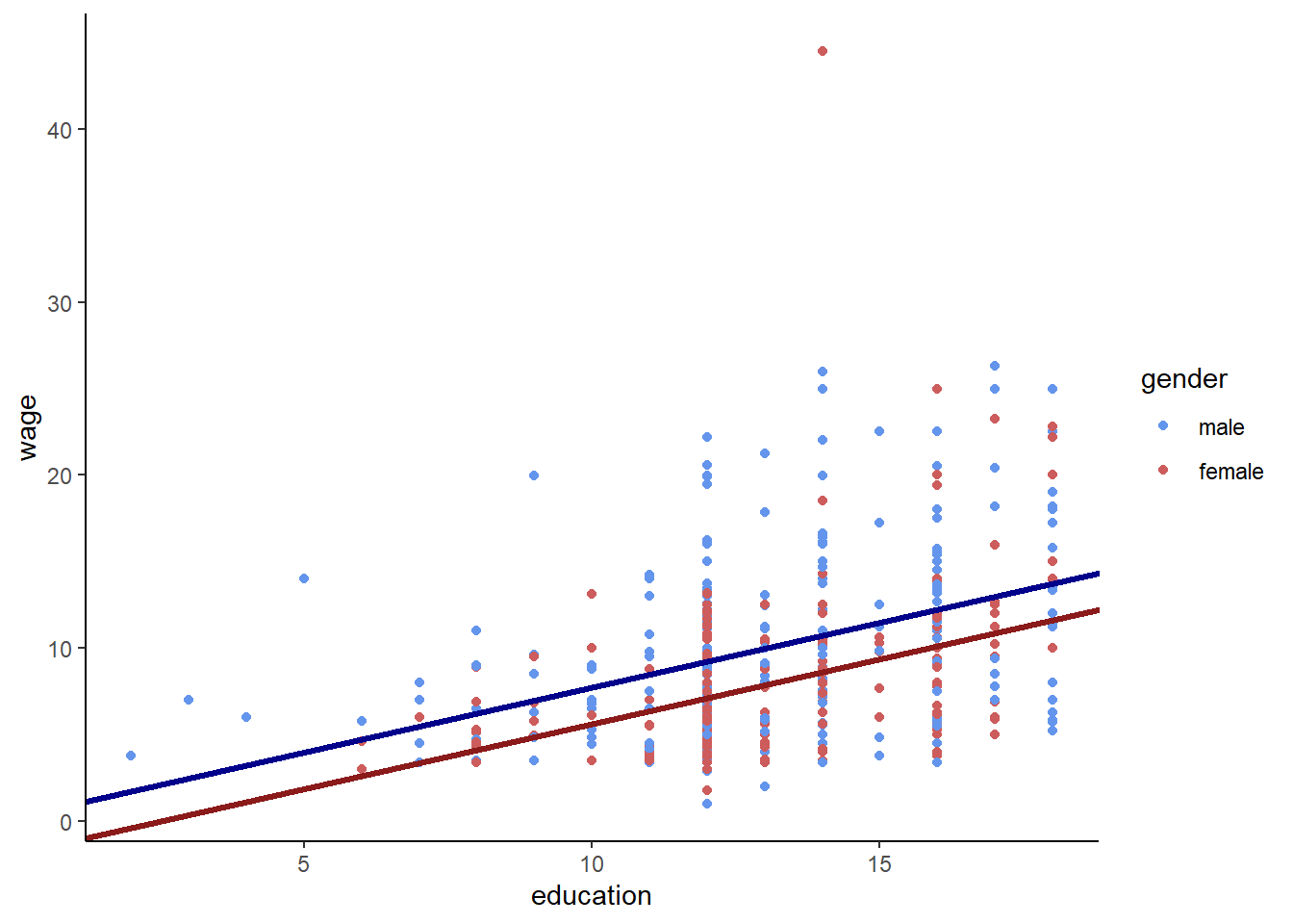
Combining categorical with numeric independent variables ias an essential tool in econometrics, so let’s work through a few more examples, starting with the AER::HousePrices data in the AER package.
As always, it is useful to look at the data helpfile (?HousePrices) to get more details on the dataset. This table has data on houses sold in Windsor, Ontario (Canada) in the summer of 1987. The data include the sales price, along with a number of attributes of each house sold, and gives us a great set of data to estimate what is called a hedonic regression. Hedonic regression is a model that attempts to predict the market value of set of goods based on the attributes of those goods, and is useful in the real world for pricing decisions. Let’s take a look at the data:
head(HousePrices)## price lotsize bedrooms bathrooms stories driveway recreation fullbase
## 1 42000 5850 3 1 2 yes no yes
## 2 38500 4000 2 1 1 yes no no
## 3 49500 3060 3 1 1 yes no no
## 4 60500 6650 3 1 2 yes yes no
## 5 61000 6360 2 1 1 yes no no
## 6 66000 4160 3 1 1 yes yes yes
## gasheat aircon garage prefer
## 1 no no 1 no
## 2 no no 0 no
## 3 no no 0 no
## 4 no no 0 no
## 5 no no 0 no
## 6 no yes 0 nosummary(HousePrices)## price lotsize bedrooms bathrooms
## Min. : 25000 Min. : 1650 Min. :1.000 Min. :1.000
## 1st Qu.: 49125 1st Qu.: 3600 1st Qu.:2.000 1st Qu.:1.000
## Median : 62000 Median : 4600 Median :3.000 Median :1.000
## Mean : 68122 Mean : 5150 Mean :2.965 Mean :1.286
## 3rd Qu.: 82000 3rd Qu.: 6360 3rd Qu.:3.000 3rd Qu.:2.000
## Max. :190000 Max. :16200 Max. :6.000 Max. :4.000
## stories driveway recreation fullbase gasheat aircon
## Min. :1.000 no : 77 no :449 no :355 no :521 no :373
## 1st Qu.:1.000 yes:469 yes: 97 yes:191 yes: 25 yes:173
## Median :2.000
## Mean :1.808
## 3rd Qu.:2.000
## Max. :4.000
## garage prefer
## Min. :0.0000 no :418
## 1st Qu.:0.0000 yes:128
## Median :0.0000
## Mean :0.6923
## 3rd Qu.:1.0000
## Max. :3.0000Let’s use price as the dependent variable, and use all of the house characteristic variables.
reg4b <- lm(price ~ lotsize + bedrooms + bathrooms + stories + driveway + recreation + fullbase + gasheat + aircon + garage + prefer, data = HousePrices)
stargazer(reg4b, type = "text")
##
## ===============================================
## Dependent variable:
## ---------------------------
## price
## -----------------------------------------------
## lotsize 3.546***
## (0.350)
##
## bedrooms 1,832.003*
## (1,047.000)
##
## bathrooms 14,335.560***
## (1,489.921)
##
## stories 6,556.946***
## (925.290)
##
## drivewayyes 6,687.779***
## (2,045.246)
##
## recreationyes 4,511.284**
## (1,899.958)
##
## fullbaseyes 5,452.386***
## (1,588.024)
##
## gasheatyes 12,831.410***
## (3,217.597)
##
## airconyes 12,632.890***
## (1,555.021)
##
## garage 4,244.829***
## (840.544)
##
## preferyes 9,369.513***
## (1,669.091)
##
## Constant -4,038.350
## (3,409.471)
##
## -----------------------------------------------
## Observations 546
## R2 0.673
## Adjusted R2 0.666
## Residual Std. Error 15,423.190 (df = 534)
## F Statistic 99.968*** (df = 11; 534)
## ===============================================
## Note: *p<0.1; **p<0.05; ***p<0.01These results have many useful, real-world applications. For example, let’s say it is the summer of 1987 and you have a house in Windsor, Ontario that you would like to sell…what is a good guess of the market price? You simply enter the attributes into the regression equation and create a prediction. For example, let’s say your house has the following characteristics:
- 5000 sqft lot
- 4 bedrooms
- 2 bathrooms
- 2 stories
- driveway
- rec room
- no basement
- no gas heating
- no air conditioning
- 2 car garage
- preferred neighborhood
We can take these attributes and put them into a new data.frame with the same variable names as in HousePrices:
yourhouse <- data.frame(lotsize = 5000, bedrooms = 4, bathrooms = 2, stories = 2, driveway = "yes", recreation = "yes", fullbase = "no", gasheat = "no", aircon = "no", garage = 2, prefer = "yes")Next, we can use the predict function and use our regression object but feed it in our custom house using the newdata option:
predict(reg4b, newdata = yourhouse)## 1
## 91864.42Such a house is predicted to sell for $91,864. Let’s take this logic a little further. Suppose your real estate agent tells you that if you want top dollar for our home, you should finish our basement, add a bedroom and a bathroom, and upgrade our HVAC to have gas heating and air conditioning. So you get a quote for all this work and it’s going to cost $35,000. We can use this model to ask the question of whether or not this work is worth it!
Let’s start by duplicating row 1 of the yourhouse dataframe into row 2:
yourhouse[2,] <- yourhouse[1,]Next, let’s edit row 2 to have the new attributes:
yourhouse[2,]$bedrooms <- 5
yourhouse[2,]$bathrooms <- 3
yourhouse[2,]$fullbase <- "yes"
yourhouse[2,]$gasheat <- "yes"
yourhouse[2,]$aircon <- "yes"
Finally, let’s rerun our prediction command:
predict(reg4b, newdata = yourhouse)## 1 2
## 91864.42 138948.66It looks like those additions would add approximately $47,000 in value to our house, so perhaps the updates are worth doing!
Let’s look at another dataset that is prime for hedonic regression, the diamonds dataset that comes in the ggplot2 package:
head(diamonds)## # A tibble: 6 x 10
## carat cut color clarity depth table price x y z
## <dbl> <ord> <ord> <ord> <dbl> <dbl> <int> <dbl> <dbl> <dbl>
## 1 0.23 Ideal E SI2 61.5 55 326 3.95 3.98 2.43
## 2 0.21 Premium E SI1 59.8 61 326 3.89 3.84 2.31
## 3 0.23 Good E VS1 56.9 65 327 4.05 4.07 2.31
## 4 0.29 Premium I VS2 62.4 58 334 4.2 4.23 2.63
## 5 0.31 Good J SI2 63.3 58 335 4.34 4.35 2.75
## 6 0.24 Very Good J VVS2 62.8 57 336 3.94 3.96 2.48summary(diamonds)## carat cut color clarity depth
## Min. :0.2000 Fair : 1610 D: 6775 SI1 :13065 Min. :43.00
## 1st Qu.:0.4000 Good : 4906 E: 9797 VS2 :12258 1st Qu.:61.00
## Median :0.7000 Very Good:12082 F: 9542 SI2 : 9194 Median :61.80
## Mean :0.7979 Premium :13791 G:11292 VS1 : 8171 Mean :61.75
## 3rd Qu.:1.0400 Ideal :21551 H: 8304 VVS2 : 5066 3rd Qu.:62.50
## Max. :5.0100 I: 5422 VVS1 : 3655 Max. :79.00
## J: 2808 (Other): 2531
## table price x y
## Min. :43.00 Min. : 326 Min. : 0.000 Min. : 0.000
## 1st Qu.:56.00 1st Qu.: 950 1st Qu.: 4.710 1st Qu.: 4.720
## Median :57.00 Median : 2401 Median : 5.700 Median : 5.710
## Mean :57.46 Mean : 3933 Mean : 5.731 Mean : 5.735
## 3rd Qu.:59.00 3rd Qu.: 5324 3rd Qu.: 6.540 3rd Qu.: 6.540
## Max. :95.00 Max. :18823 Max. :10.740 Max. :58.900
##
## z
## Min. : 0.000
## 1st Qu.: 2.910
## Median : 3.530
## Mean : 3.539
## 3rd Qu.: 4.040
## Max. :31.800
## This dataset includes information about over 50,000 round cut diamonds; let’s use a hedonic pricing model to estimate diamond price as a function of the 4 C’s of diamonds:
- Carat
- Cut
- Color
- Clarity
Carat is the weight of the diamond, so it is a number. However, cut, color, and clarity are all categorical (factor) variables with lots of levels, so this is going to be a big dummy variable regression.
For ease of reading the output tables, we will first force R to read the categorical variables as unordered. Then we run a regression with the 4 C’s as above, as well as with a squared term for diamond size:
diamonds2 <- as.data.frame(diamonds)
diamonds2$cut <- factor(diamonds2$cut, ordered = FALSE)
diamonds2$color <- factor(diamonds2$color, ordered = FALSE)
diamonds2$clarity <- factor(diamonds2$clarity, ordered = FALSE)
diamonds2$color <- relevel(diamonds2$color, c("J"))
reg4c <- lm(price ~ carat +I(carat^2) + cut + color + clarity, data = diamonds2)
stargazer(reg4c, type = "text")
##
## ==================================================
## Dependent variable:
## ------------------------------
## price
## --------------------------------------------------
## carat 8,011.170***
## (35.989)
##
## I(carat2) 408.236***
## (15.837)
##
## cutGood 655.285***
## (33.429)
##
## cutVery Good 840.755***
## (31.088)
##
## cutPremium 852.509***
## (30.749)
##
## cutIdeal 977.763***
## (30.480)
##
## colorD 2,350.917***
## (26.578)
##
## colorE 2,140.301***
## (25.346)
##
## colorF 2,066.280***
## (25.244)
##
## colorG 1,861.515***
## (24.744)
##
## colorH 1,377.922***
## (25.336)
##
## colorI 899.174***
## (26.799)
##
## claritySI2 2,702.286***
## (44.614)
##
## claritySI1 3,657.520***
## (44.445)
##
## clarityVS2 4,284.790***
## (44.644)
##
## clarityVS1 4,599.649***
## (45.327)
##
## clarityVVS2 5,006.760***
## (46.630)
##
## clarityVVS1 5,088.823***
## (47.921)
##
## clarityIF 5,433.013***
## (51.821)
##
## Constant -9,421.919***
## (56.227)
##
## --------------------------------------------------
## Observations 53,940
## R2 0.917
## Adjusted R2 0.917
## Residual Std. Error 1,149.800 (df = 53920)
## F Statistic 31,338.700*** (df = 19; 53920)
## ==================================================
## Note: *p<0.1; **p<0.05; ***p<0.01Could we predict the price of a 32 carat, D color, internally flawless with ideal cut diamond? Mathematically, sure we could:
mydiamond <- data.frame(carat = 32, clarity = "IF", cut = "Ideal", color = "D")
predict(reg4c, newdata = mydiamond)
## 1
## 673731.4But statistically this is a bad idea. If we look at a summary of the data:
summary(diamonds2$carat)## Min. 1st Qu. Median Mean 3rd Qu. Max.
## 0.2000 0.4000 0.7000 0.7979 1.0400 5.0100We see that the biggest diamond in the data set was only 5.01 carats. Thus, making a prediction about a 32 carat diamond is beyond the scope of the model, as the prediction is trying to estimate a point outside of the range of the sample data. This is called extrapolation and is generally frowned upon; we may be fairly sure that the relationship between size and price is linear in the range we are looking at, there is no guarantee that it is linear beyond the range of the data (and in the case of diamonds, it almost certainly is not!). This is also, generally speaking, why the intercept is not often of practical importance!
Figure 7.1: XKCD: Extrapolating
Turning away from hedonic regression, let’s look at the gpa2 data in the wooldridge package. Let’s model GPA as a function of SAT score, an athlete dummy, and a gender dummy. Note that this data set has the athlete and gender variables coded as dummies already, so we are not dealing with factor variables. Additionally, for better interpretability I rescale the SAT variable by dividing it by 100–this means we interpret the results as a 100 point change rather than a 1 point change.
reg4d <- lm(colgpa ~ I(sat/100) + athlete + female, data = gpa2)
stargazer(reg4d, type = "text")
##
## ===============================================
## Dependent variable:
## ---------------------------
## colgpa
## -----------------------------------------------
## I(sat/100) 0.206***
## (0.007)
##
## athlete 0.020
## (0.045)
##
## female 0.232***
## (0.019)
##
## Constant 0.421***
## (0.073)
##
## -----------------------------------------------
## Observations 4,137
## R2 0.197
## Adjusted R2 0.196
## Residual Std. Error 0.591 (df = 4133)
## F Statistic 337.404*** (df = 3; 4133)
## ===============================================
## Note: *p<0.1; **p<0.05; ***p<0.01These results suggest:
- For each additional 100 points on the SAT, the model predicts a (statistically significant) .2 increase in GPA. This effect is assumed to be the same for males and females, athletes and non-athletes.
- The average GPA among athletes is 0.02 higher than for non-athletes. This difference is not statistically significant.
- Females have on average a .23 higher GPA than males. This difference is statistically significant.
Lets try this again with a slight variation: here we include a female athlete interaction effect.
reg4e <- lm(colgpa ~ I(sat/100) + athlete*female, data = gpa2)
stargazer(reg4d, reg4e, type = "text")
##
## =======================================================================
## Dependent variable:
## ---------------------------------------------------
## colgpa
## (1) (2)
## -----------------------------------------------------------------------
## I(sat/100) 0.206*** 0.206***
## (0.007) (0.007)
##
## athlete 0.020 0.003
## (0.045) (0.051)
##
## female 0.232*** 0.229***
## (0.019) (0.019)
##
## athlete:female 0.071
## (0.102)
##
## Constant 0.421*** 0.424***
## (0.073) (0.073)
##
## -----------------------------------------------------------------------
## Observations 4,137 4,137
## R2 0.197 0.197
## Adjusted R2 0.196 0.196
## Residual Std. Error 0.591 (df = 4133) 0.591 (df = 4132)
## F Statistic 337.404*** (df = 3; 4133) 253.142*** (df = 4; 4132)
## =======================================================================
## Note: *p<0.1; **p<0.05; ***p<0.01Note that R includes both the interaction variable, as well as the two variables individually. This is exactly what you want it to do.
Judging from the lack of significance of the interaction term and the fact that the adjusted \(R^2\) did not move, it seems like there is no interaction effect. This implies that the effect of gender on grades is not affected by one’s status of being an athlete (or equivalently, the effect of being an athlete is not different between males and females).
Let’s examine one more example involving interaction effects before moving on with the TeachingRatings data set from the AER package. We will estimate a regression looking at the relationship between student evaluation of instructors and the attractiveness of instructors, dummies for minority and female faculty (one model interacts them), a native english speaker dummy, and a dummy to indicate whether or not the class is a single credit elective course (e.g. yoga):
reg4f <- lm(eval~beauty + gender + minority + native + credits, data = TeachingRatings)
reg4g <- lm(eval~beauty + gender*minority + native + credits, data = TeachingRatings)
stargazer(reg4f, reg4g, type = "text")
##
## ========================================================================
## Dependent variable:
## -----------------------------------------------
## eval
## (1) (2)
## ------------------------------------------------------------------------
## beauty 0.166*** 0.175***
## (0.031) (0.031)
##
## genderfemale -0.174*** -0.140***
## (0.049) (0.052)
##
## minorityyes -0.165** -0.003
## (0.076) (0.116)
##
## nativeno -0.248** -0.289***
## (0.105) (0.107)
##
## creditssingle 0.641*** 0.597***
## (0.106) (0.109)
##
## genderfemale:minorityyes -0.271*
## (0.147)
##
## Constant 4.072*** 4.061***
## (0.033) (0.033)
##
## ------------------------------------------------------------------------
## Observations 463 463
## R2 0.155 0.161
## Adjusted R2 0.145 0.150
## Residual Std. Error 0.513 (df = 457) 0.512 (df = 456)
## F Statistic 16.711*** (df = 5; 457) 14.563*** (df = 6; 456)
## ========================================================================
## Note: *p<0.1; **p<0.05; ***p<0.01Let’s look specifically at the interacted variables. The function of an interaction effect is really to give an it depends sort of answer. If I were to ask the question, do minority faculty receive lower teaching evaluations, the answer to that question is that it depends on if whether or not that faculty is male or female. A minority male would have a 1 for the minority dummy, but a 0 for the interaction dummy, so in aggregate he would be expected to receive a teaching evaluation, all else equal, that is .003 lower than the omitted group (here, that is non-minority males). However, a minority female would receive a 1 for the minority dummy, the female dummy, AND the interaction dummy, so she would be expected to receive a teaching evaluation (again all else equal) .414 lower than a non-minority male and 0.274 lower than a non-minority female.
Another question you might ask here is whether or not you should bother keeping the minority dummy at all and just roll with the interaction dummy and the female dummy. After all, the minority dummy is basically 0 and nowhere close to significant. The answer here is that yes, you absolutely need to keep that dummy. The idea behind this is called the principle of marginality, which basically states that if an independent variable in your regression is either a) an interaction effect, or b) a “higher power” of a variable in the model (e.g. a squared term), then you should include the variables from which they are derived in the model. So in this case, this means if you interact the \(female\) and \(minority\) variables, you need to keep both \(female\) and \(minority\) in the model if you have the interaction effect in the model. Similarly, if in the hedonic regression above using the diamonds data it turned out the that squared term was significant but the linear term was not, we still ougut to keep the linear term in the model.
7.4 Interactions with Numeric Variables
In this section, we will look at interactions with numeric variables. Interpreting these can be tricky, but remember, the overall intuition behind interaction effects remains the same–we believe that the relationship between the dependent varaible \(Y\) and an independent variable \(X_1\) depends on some other variable \(X_2\).
Let’s take a look at the CPS1988 data and estimate a regression with log of wages as our dependent variable and experience, experience squared, and an interaction between years of education (a numeric variable) and ethnicity (a factor variable) as our independent variables. The interaction effect means that we are looking for an it depends kind of answer to the question of what is the relationship between years of education and wages and does it depend on whether or not somebody is white or black.
reg5a <- lm(log(wage) ~ experience + I(experience^2) + education*ethnicity, data = CPS1988)
stargazer(reg5a, type = "text")
##
## ====================================================
## Dependent variable:
## ----------------------------
## log(wage)
## ----------------------------------------------------
## experience 0.078***
## (0.001)
##
## I(experience2) -0.001***
## (0.00002)
##
## education 0.086***
## (0.001)
##
## ethnicityafam -0.124**
## (0.059)
##
## education:ethnicityafam -0.010**
## (0.005)
##
## Constant 4.313***
## (0.020)
##
## ----------------------------------------------------
## Observations 28,155
## R2 0.335
## Adjusted R2 0.335
## Residual Std. Error 0.584 (df = 28149)
## F Statistic 2,834.022*** (df = 5; 28149)
## ====================================================
## Note: *p<0.1; **p<0.05; ***p<0.01Interpreting this regression requires us to combine a lot of things we have learned already:
- First, recall that using the log term for wages affects our interpretation of the coefficients!
- The fact that the linear term on experience has a positive sign and the squared term has a negative sign indicates decreasing returns to experience: more experience leads to higher wages, but earlier years have a larger marginal effect on wages than later years.
Let’s dig deeper into the interaction effect and start off by writing out the entire regression model:
\[\begin{equation} ln(Wage_{i}) = 4.313 + 0.078 \cdot experience_i - .001 \cdot experience_i^2 - 0.124 \cdot ethnicity_i + .086 \cdot education_i - .010 \cdot education_i \cdot ethnicity_i \end{equation}\]
Let’s simplify our discussion by assuming the individual in question has 10 years of experience, so the first three terms can be simplified as \(4.313 + 0.078 \cdot 10 - 0.001 \cdot 10^2 = 4.993\). We can plug this into our model, so now:
\[\begin{equation} ln(Wage_{i}) = 4.993 - 0.124 \cdot ethnicity_i + .086 \cdot education_i - .010 \cdot education_i \cdot ethnicity_i \end{equation}\]
The ethnicity variable has two levels, “cauc” (Caucasian) and “afam” (African American). In this model, \(ethnicity_i = 1\) for observations identified in the data as African American and \(ethinicity_i = 0\) for observations coded as Caucasian, so Caucasian is the omitted group and African American is the included group.
If we plug \(ethnicity_i = 1\) into that equation, we get the regression line for African Americans, which simplifies to:
\[\begin{equation} ln(Wage_{i}) = 4.993 - 0.124 + .086 \cdot education_i - .010 \cdot education_i ln(Wage_{i}) = 4.869 + 0.076 \cdot education_i \end{equation}\]
If we plug in \(ethnicity_i = 0\) for Caucasians, we get:
\[\begin{equation} ln(Wage_{i}) = 4.993 + .086 \cdot education_i \end{equation}\]
For African Americans, both the intercept is different (due to the \(\hat{\beta}\) on the ethnicity dummy), and the slope on education is different (due to the \(\hat{\beta}\) on the interaction effect). Reminding ourselves of the regression results:
##
## ====================================================
##                             Dependent variable:
##                         ----------------------------
##                                  log(wage)
## ----------------------------------------------------
## experience                        0.078***
##                                   (0.001)
##
## I(experience2)                   -0.001***
##                                  (0.00002)
##
## education                         0.086***
##                                   (0.001)
##
## ethnicityafam                     -0.124**
##                                   (0.059)
##
## education:ethnicityafam           -0.010**
##                                   (0.005)
##
## Constant                          4.313***
##                                   (0.020)
##
## ----------------------------------------------------
## Observations                       28,155
## R2                                 0.335
## Adjusted R2                        0.335
## Residual Std. Error          0.584 (df = 28149)
## F Statistic             2,834.022*** (df = 5; 28149)
## ====================================================
## Note: *p<0.1; **p<0.05; ***p<0.01The negative \(\hat{\beta}\) on the interaction effect is telling us that the marginal effect of an additional year of education appears to be slightly lower for African Americans than it is for Caucasians – the point estimates imply an 7.6% increase in wages per year of education for African Americans vs 8.6% per year for Caucasians.
It is possible, though not terribly common, to estimate interaction effects between two numeric variables. Let’s consider a model we looked at in Chapter 5, looking at the relationship between school funding and test scores in the meap01 data set:
reg5b <- lm(math4 ~ exppp + lunch, data = meap01)
stargazer(reg5b, type = "text")
##
## ===============================================
## Dependent variable:
## ---------------------------
## math4
## -----------------------------------------------
## exppp 0.002***
## (0.0004)
##
## lunch -0.471***
## (0.014)
##
## Constant 79.568***
## (1.813)
##
## -----------------------------------------------
## Observations 1,823
## R2 0.368
## Adjusted R2 0.368
## Residual Std. Error 15.867 (df = 1820)
## F Statistic 530.804*** (df = 2; 1820)
## ===============================================
## Note: *p<0.1; **p<0.05; ***p<0.01In this regression, we saw that higher poverty rates were correlated with lower math scores, while higher levels of funding were correlated with higher math scores. Perhaps your theory is that there ought to be an interaction between these variables; for example, maybe you believe that increases in funding should be more important in poor schools. we could test this by interacting the exppp and lunch variables:
reg5c <- lm(math4 ~ exppp * lunch, data = meap01)
stargazer(reg5b, reg5c, type = "text")
##
## =======================================================================
## Dependent variable:
## ---------------------------------------------------
## math4
## (1) (2)
## -----------------------------------------------------------------------
## exppp 0.002*** 0.002***
## (0.0004) (0.001)
##
## lunch -0.471*** -0.424***
## (0.014) (0.071)
##
## exppp:lunch -0.00001
## (0.00001)
##
## Constant 79.568*** 77.690***
## (1.813) (3.330)
##
## -----------------------------------------------------------------------
## Observations 1,823 1,823
## R2 0.368 0.369
## Adjusted R2 0.368 0.368
## Residual Std. Error 15.867 (df = 1820) 15.869 (df = 1819)
## F Statistic 530.804*** (df = 2; 1820) 353.914*** (df = 3; 1819)
## =======================================================================
## Note: *p<0.1; **p<0.05; ***p<0.01If your theory were correct, you would expect to see a positive and significant sign on the interaction term. However, the interaction term is the wrong sign to support that theory and insignificant as well, suggesting that perhaps the impact of funding is not different based on the poverty characteristics of schools.
Generally speaking, interpreting interactions between numeric variables is quite trick. This is often a case where you only interpret the sign of the coefficient due to how difficult they are to interpret numerically.
7.5 Wrapping up
When we began our discussion of regression, we limited ourselves to using only numeric independent variables; in this chapter, we extended power of regression modeling can be extended to include categorical independent variables as well. The next step is to consider the ability of regression modeling to explain categorical dependent variables.
7.6 End of Chapter Exercises
Model Building: For each of the following, examine the data (and the help file for the data) to try and build a good multivariate regression. Think carefully about the variables you have to choose among to explain your dependent variable with. Ensure that you include both categorical and numeric variables in your regression, consider strongly the use of non-linear or interaction effects in your model. Finally, interpret your results, and note that some of the variables suggested as dependent variables are in log form which affects their interpretation.
AER:GrowthDJ- look at economic growth.AER:CollegeDistance- use \(education\) as the dependent variable.wooldridge:beauty- use \(wage\) or \(logwage\) as your dependent variable.wooldridge:campus- Use some measure of crime as your dependent variable. It might be worth transforming some variables into rate variables (e.g. divide the number of crimes by the number of people so you can fairly compare large schools with small schools).wooldridge:twoyear- This data looks at the returns to education from 2 and 4 year colleges, use the \(lwage\) variable (log wages) as your dependent variable.Choose any of one of the
wooldridgedatasets relating to gpa:gpa,gpa2, orgpa3and predict GPA.