Chapter 6 Regression Assumptions
The OLS model encountered in Chapter 5 is built on a series of assumptions that we will now examine. We will also look at some of the tools at our disposal when one or more of the assumptions do not hold. As usual, I start with loading in the data I will be using. Additionally, there are a couple new libraries introduced in this chapter: lmtest and sandwich. If they are not installedon your computer, You will need to use the install.packages() function on them first. Finally, I will no longer be using the convention of attaching datasets. My general feeling is that it is not best practice anyhow, but more practically, there are a few datasets in this chapter that have clashing variable names, which would make the analysis messy.
data(wage1)
data(CPS1985)
data(ceosal1)
data(nyse)
data(smoke)
data(vote1)
data(hprice3)
data(infmrt)
We will work through a series of assumptions upon which the OLS model is built, and what one might do if these assumptions do not hold.
6.1 Assumption 1: The Linear Regression Model is “Linear in Parameters”
The basic model is:
\[\begin{equation} Y_{i} = \alpha + \beta X_{i} + \epsilon_i \end{equation}\]
This is the equation for a straight line. But what if the data doesn’t really look like a straight line? Let’s look at this data from the ceosal1 dataset in the wooldridge package. Here, we graph CEO salary on the Y axis and the company sales on the X axis.
ceosal1 %>% ggplot(aes(y = salary, x = sales)) +
    geom_point() +
    theme_classic() +
    geom_smooth(method=lm)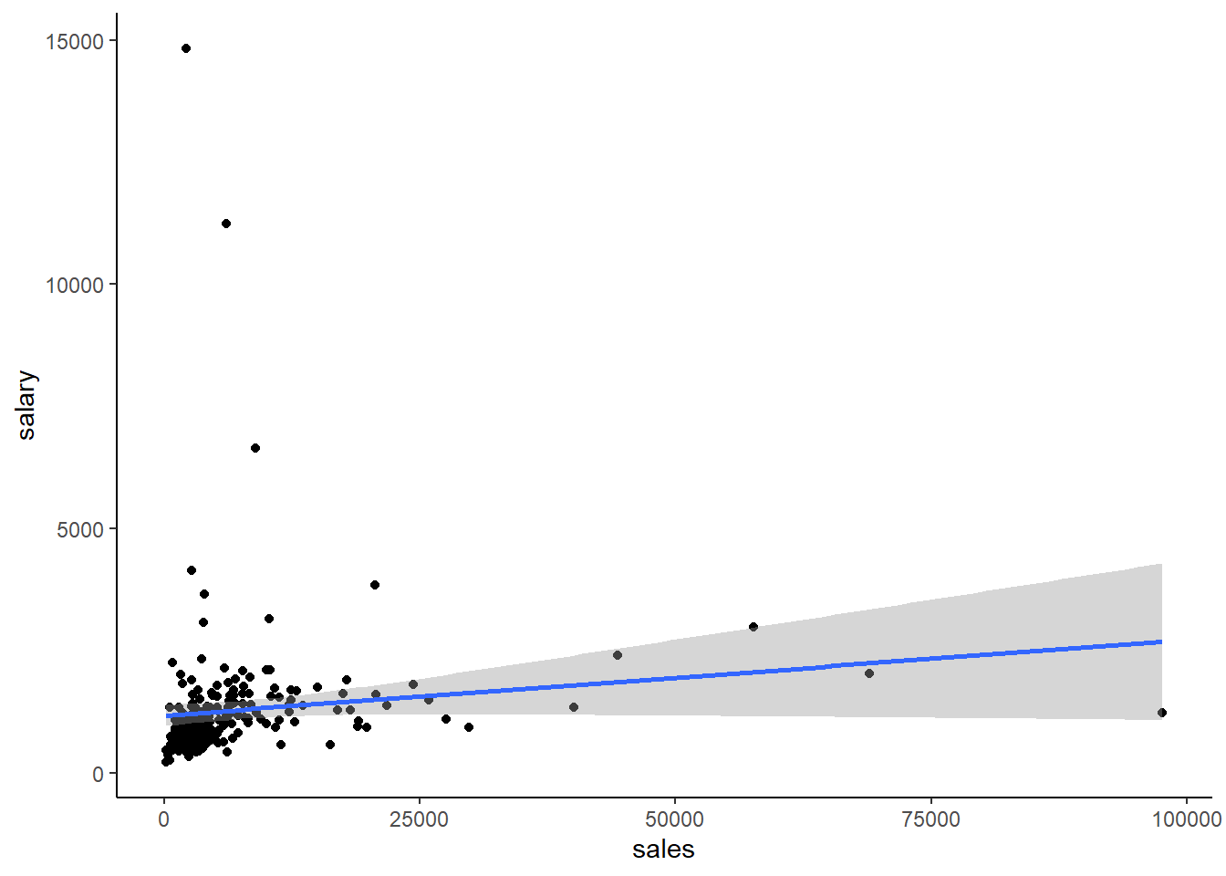
So this doesn’t say much, and I’d guess there is not much of a relationship when we estimate the regression. But, part of what is going on might be due to the fact that both the CEO salary and sales data look skewed, so maybe we just don’t have a linear relationship. Let’s see what the regression looks like:
reg1a <- lm(salary ~ sales, data = ceosal1)
stargazer(reg1a, type = "text")
##
## ===============================================
## Dependent variable:
## ---------------------------
## salary
## -----------------------------------------------
## sales 0.015*
## (0.009)
##
## Constant 1,174.005***
## (112.813)
##
## -----------------------------------------------
## Observations 209
## R2 0.014
## Adjusted R2 0.010
## Residual Std. Error 1,365.737 (df = 207)
## F Statistic 3.018* (df = 1; 207)
## ===============================================
## Note: *p<0.1; **p<0.05; ***p<0.01The result is significant at the 10% level, \(R^2 = .01\) is tiny, but we might be able to do better if we do something about the non-linearity.
All OLS requires is that the model is linear in parameters. We can take what we learned in Chapter 5 about data transformation to do some mathematical transformations of the data to create a linear function. Here, let’s calculate the natural log of both salary and sales and plot them.
tempdata <- ceosal1 %>%
    mutate(lnsalary = log(salary)) %>%
    mutate(lnsales = log(sales))
Now, let’s take a look at the plot between lnsales and lnprice:
tempdata %>% ggplot(aes(x = lnsales, y = lnsalary)) +
    geom_point() +
    theme_classic() +
  geom_smooth(method = lm)
## `geom_smooth()` using formula 'y ~ x'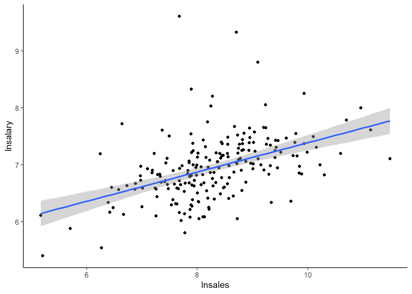
This is quite a change from the previous graph! In fact, this data looks like it might actually have a linear relationship now.
reg1b <- lm(lnsalary ~ lnsales, data = tempdata)
stargazer(reg1b, type = "text")
##
## ===============================================
## Dependent variable:
## ---------------------------
## lnsalary
## -----------------------------------------------
## lnsales 0.257***
## (0.035)
##
## Constant 4.822***
## (0.288)
##
## -----------------------------------------------
## Observations 209
## R2 0.211
## Adjusted R2 0.207
## Residual Std. Error 0.504 (df = 207)
## F Statistic 55.297*** (df = 1; 207)
## ===============================================
## Note: *p<0.1; **p<0.05; ***p<0.01The \(R^2\) is considerably higher now, the \(\beta\) is significant at the 1% level, and all in all this is a much more compelling model.
The log transformation is probably the most common one we see in econometrics. Not only because it is useful in making skewed data more amenable to linear approaches, but because there is a very useful interpretation of the results. Let’s look at the regressions again, side by side:
stargazer(reg1a, reg1b, type = "text")##
## ===========================================================
## Dependent variable:
## ----------------------------
## salary lnsalary
## (1) (2)
## -----------------------------------------------------------
## sales 0.015*
## (0.009)
##
## lnsales 0.257***
## (0.035)
##
## Constant 1,174.005*** 4.822***
## (112.813) (0.288)
##
## -----------------------------------------------------------
## Observations 209 209
## R2 0.014 0.211
## Adjusted R2 0.010 0.207
## Residual Std. Error (df = 207) 1,365.737 0.504
## F Statistic (df = 1; 207) 3.018* 55.297***
## ===========================================================
## Note: *p<0.1; **p<0.05; ***p<0.01The regression on the left was the linear-linear model. Interpreting this coefficient demands that we are aware of the units of measure in the data: sales are measured in millions of dollars, salary in thousands of dollars. So \(\beta=0.015\) literally says that if sales goes up by 1, salary goes up by 0.015. But we interpret this as saying that, for every additional $1,000,000 in sales, CEO salary is expected to go up by $15. The model on the right is the log-log model. By log transforming a variable before estimating the regression, you change the interpretation from level increases into percentage increases. This model states that a 1% increase in sales on average leads to CEO pay going up by 0.257%.
Let’s look at the linear-log and log-linear models too.
reg1c <- lm(lnsalary ~ sales, data = tempdata)
reg1d <- lm(salary ~ lnsales, data = tempdata)
stargazer(reg1a, reg1d, reg1c, reg1b, type = "text")
##
## ===========================================================================
## Dependent variable:
## --------------------------------------------
## salary lnsalary
## (1) (2) (3) (4)
## ---------------------------------------------------------------------------
## sales 0.015* 0.00001***
## (0.009) (0.00000)
##
## lnsales 262.901*** 0.257***
## (92.355) (0.035)
##
## Constant 1,174.005*** -898.929 6.847*** 4.822***
## (112.813) (771.502) (0.045) (0.288)
##
## ---------------------------------------------------------------------------
## Observations 209 209 209 209
## R2 0.014 0.038 0.079 0.211
## Adjusted R2 0.010 0.033 0.075 0.207
## Residual Std. Error (df = 207) 1,365.737 1,349.496 0.545 0.504
## F Statistic (df = 1; 207) 3.018* 8.103*** 17.785*** 55.297***
## ===========================================================================
## Note: *p<0.1; **p<0.05; ***p<0.01Here all 4 specifications are side-by-side. We’ve already interpreted columns 1 and 4. How would we interpret columns 2 and 3?
Column 2 is the linear-log model (\(salary\) is linear, \(sales\) is logged). A 1% increase in sales is associated with an increase in CEO salary of $2,629.01 (there’s some calculus involved here, but the shortcut is just to move the decimal place 2 spaces to the left).
Column 3 is the log-linear model. A $1,000,000 increase in sales is associated with a .1% higher salary (again, there’s some calculus involved here, but the shortcut here is to move the decimal place 2 spaces to the right).
The model in column 4 seems to be the best model of the bunch.
Another common non-linear transformation is the quadratic transformation; this is particularly useful in cases where you think a relationship may be decreasing up to a point, and then start increasing after that point (or vice versa). To see this in action, let’s look at a graph that looks at the relationship between the age and selling prices of homes in the hprice3 data from the wooldridge package.
hprice3 %>% ggplot(aes(x = age, y = price)) +
    geom_point(color = "cornflowerblue") +
    theme_classic() +
labs(title = "House Value and Age") 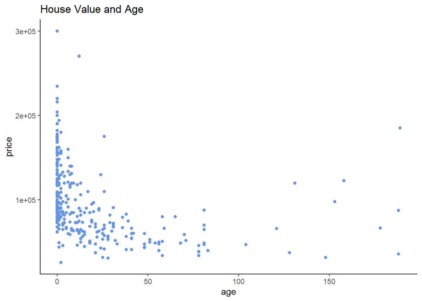
This relationship looks somewhat U-shaped; moving left to right, it seems that the value of houses falls as they get older, but at a certain point, the relationship reverses course and older becomes more valuable!
This is a great place to estimate a quadratic regression, which is just a fancy term for including both \(age\) and \(age^2\) in our regression.
\[\begin{equation} Price_{i} = \alpha + \beta_1 age_{i} + \beta_2 age_i^2 + \epsilon_i \end{equation}\]
The best method here is to include the I() argument in our regression; alternately, we can manually create a squared term and put it in our regression. The hprice3 data already has a squared term in it called agesq, so let’s verify that both methods get us to the same place:
reg1e <- lm(price ~ age, data = hprice3)
reg1f <- lm(price ~ age + I(age^2), data = hprice3)
reg1g <- lm(price ~ age + agesq, data = hprice3)
stargazer(reg1e, reg1f, reg1g, type = "text")
##
## ===========================================================================================
## Dependent variable:
## -----------------------------------------------------------------------
## price
## (1) (2) (3)
## -------------------------------------------------------------------------------------------
## age -440.566*** -1,690.903*** -1,690.903***
## (70.100) (157.309) (157.309)
##
## I(age2) 9.258***
## (1.067)
##
## agesq 9.258***
## (1.067)
##
## Constant 104,035.000*** 113,762.100*** 113,762.100***
## (2,605.563) (2,600.544) (2,600.544)
##
## -------------------------------------------------------------------------------------------
## Observations 321 321 321
## R2 0.110 0.281 0.281
## Adjusted R2 0.107 0.276 0.276
## Residual Std. Error 40,836.920 (df = 319) 36,777.670 (df = 318) 36,777.670 (df = 318)
## F Statistic 39.499*** (df = 1; 319) 62.002*** (df = 2; 318) 62.002*** (df = 2; 318)
## ===========================================================================================
## Note: *p<0.1; **p<0.05; ***p<0.01Both columns 2 and 3 are the same, as expected. Our regression model, then, looks like:
\[\begin{equation} Price_{i} = \$113,762.10 - \$1691.90 age_{i} + \$9.26 age_i^2 + \epsilon_i \end{equation}\]
We can look at these two models graphically as well: the green line is the linear model (column 1 above), the red line is the quadratic model (column 2/3 above). The red line is clearly a better fit.
hprice3 %>% ggplot(aes(x = age, y = price)) +
    geom_point(color = "cornflowerblue",
               alpha = .4) +
    theme_classic() +
    labs(title = "House Value and Age",
         y = "Price",
         x = "Age") +
    geom_smooth(method = lm,
                color = "palegreen4",
                se = FALSE) +
    geom_smooth(method = lm,
                formula = y ~ x + I(x^2),
                color = "indianred3",
                se = FALSE) +
    scale_y_continuous(labels=scales::dollar_format())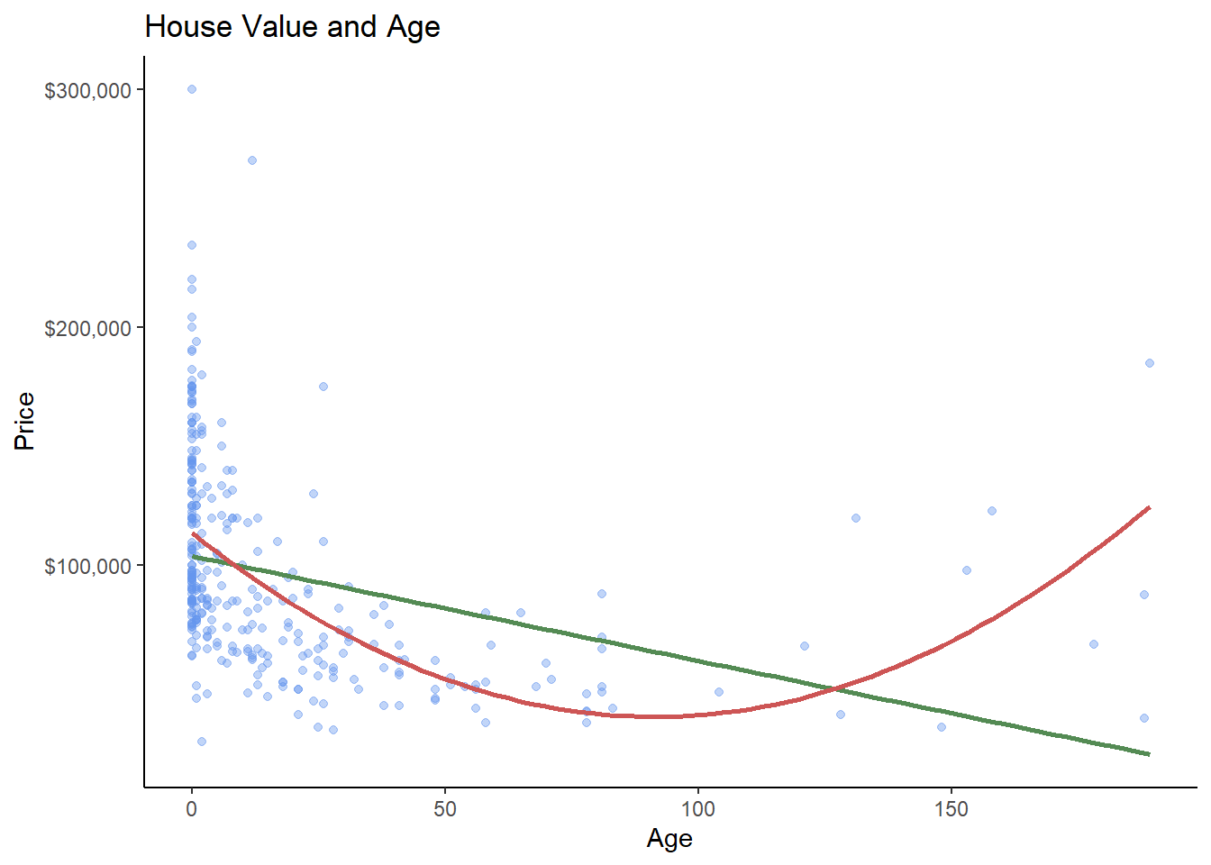
We can also, with a little bit of calculus, figure out the age at which the relationship stops decreasing and starts increasing. You simply need to take the derivative of the regression equation with respect to age, set it equal to zero, and solve for age!
\[\begin{equation} Price_{i} = \$113,762.10 - \$1691.90 age_{i} + \$9.26 age_i^2 + \epsilon_i \end{equation}\] \[\begin{equation} \frac{\partial Price_i}{\partial age} = \$1691.90 + 2 \cdot \$9.26 age_i = 0 \: at \: age^\star \end{equation}\] \[\begin{equation} \frac{\$1691.90}{\$18.52} = age^\star=91.4 \end{equation}\]
As houses in this dataset age, they lose value until they hit 91.4 years of age, at which point they start appreciating in value!
6.2 Assumption 2: The Average of the Error Term is 0
You may have wondered why we bother with having a constant term \(\alpha\) in our regressions if nobody really cares about it. It turns out that the constant term is what makes this assumption true. For example. let’s look back at our log-log model from the above:
summary(reg1b)##
## Call:
## lm(formula = lnsalary ~ lnsales, data = tempdata)
##
## Residuals:
## Min 1Q Median 3Q Max
## -1.01038 -0.28140 -0.02723 0.21222 2.81128
##
## Coefficients:
## Estimate Std. Error t value Pr(>|t|)
## (Intercept) 4.82200 0.28834 16.723 < 2e-16 ***
## lnsales 0.25667 0.03452 7.436 2.7e-12 ***
## ---
## Signif. codes: 0 '***' 0.001 '**' 0.01 '*' 0.05 '.' 0.1 ' ' 1
##
## Residual standard error: 0.5044 on 207 degrees of freedom
## Multiple R-squared: 0.2108, Adjusted R-squared: 0.207
## F-statistic: 55.3 on 1 and 207 DF, p-value: 2.703e-12The Residuals panel looks at the distribution of the error term. Each residual from the regression is stored in the regression object; let’s put them in our tempdata dataset and take a look at the first few rows.
tempdata$resid <- reg1b$residuals
head(tempdata[c(1,3,13,14,15)],)
## salary sales lnsalary lnsales resid
## 1 1095 27595.0 6.998510 10.225390 -0.44805495
## 2 1001 9958.0 6.908755 9.206132 -0.27619505
## 3 1122 6125.9 7.022868 8.720281 -0.03737765
## 4 578 16246.0 6.359574 9.695602 -0.95100918
## 5 1368 21783.2 7.221105 9.988894 -0.16475777
## 6 1145 6021.4 7.043160 8.703075 -0.01266956Is the mean of our residuals = 0?
mean(tempdata$resid)## [1] 2.638171e-17I mean…that’s about as close to zero as you can get:
format(mean(tempdata$resid), scientific = FALSE)## [1] "0.00000000000000002638171"As long as you always have \(\alpha\) in your regression, this assumption isn’t something to worry about. There are only occasionally cases where you might want to run a regression without a constant, but they are rare.
6.4 Assumption 4: The Error Term is not Serially Correlated.
This is mostly a problem in time series regression (a regression where you use a continuous measure of time as an independent variable), and refers to a situation in which you can use error terms to predict each other. Let’s take a look at this data from the New York Stock Exchange from the wooldridge package–these data are about 12 years of Wednesday closing prices of the NYSE. The helpfile doesn’t specify when the data is from, but since the data includes a pretty big market crash around observation 620 or so, I will speculate that this data is from the 1980s and the huge drop is in October, 1987.
tempdata2 <- nyse
tempdata2 %>% ggplot(aes(x = t, y = price)) +
geom_point() +
geom_line()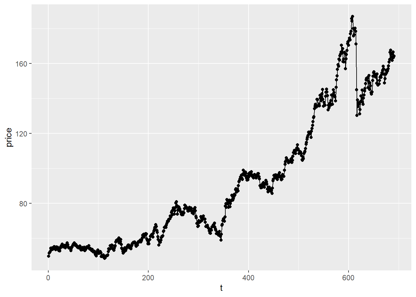 Next, let’s estimate the regression and plot the residuals on the Y axis against time:
reg4a <- lm(price ~ t, data = tempdata2)
tempdata2$resid <- reg4a$residuals
tempdata2 %>% ggplot(aes(x = t, y = resid)) +
    geom_point() +
    geom_line()
This graph exhibits what is called serial correlation or autocorrelation as the error terms are correlated with each other. In other words, if we know the error term for week 1, we can use that to make a pretty good guess about the error term for week 2, and so forth.
Again, the issues of serial correlation are mostly time series issues, so we will take a deeper look at these in Chapter 10.
6.5 Assumption 5: Homoskedasticity of the Error Term
We assume that the error term is homoskedastic, which means that the variance of the error term is not correlated with the dependent variable. If the variance of the error term is correlated with the dependent variable, the data is said to be heteroskedastic. We can look for heteroskedasticity by looking at a plot of residuals and fitted values.

Let’s take a look at a regression with homoskedasticity first. In Chapter 5 we looked at the voting share data from vote1; here, we estimate the regression and plot the fitted values on the X-axis and the residuals on the Y-axis. For ease of reading, I am adding a horizontal line at 0:
reg5a <- lm(voteA ~ shareA, data = vote1)
plot(reg5a$residuals ~ reg5a$fitted.values)
abline(a = 0, b = 0)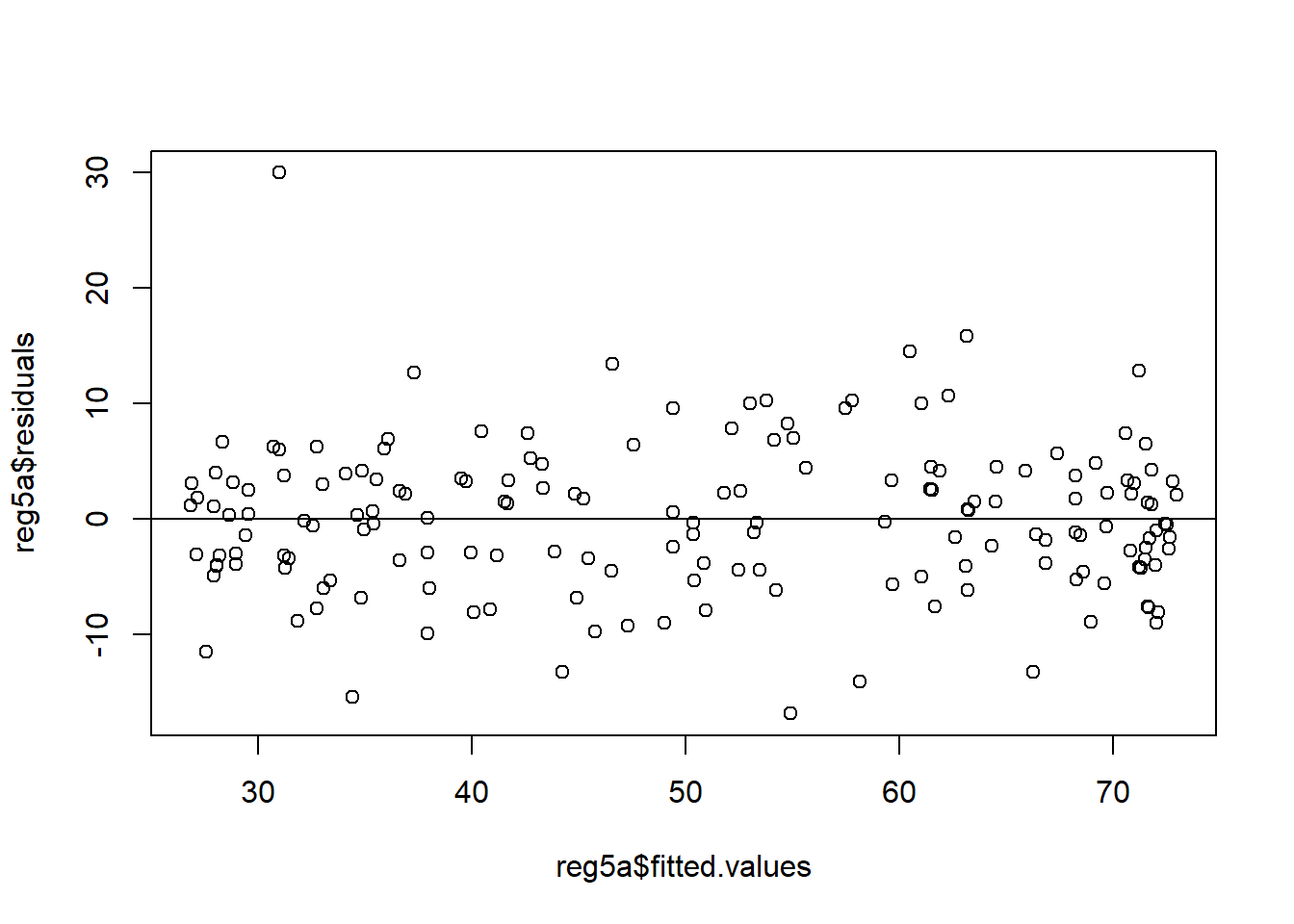
Note that the variation around the horizontal line is roughly the same for all of the possible fitted values. In other words, that 0 line that I added may very well be the line of best fit if I ran a regression!
Now, let’s take a look at a regression using the smoke data in the wooldridge package. We estimate the effect of \(income\) on the number of daily cigarettes smoked, \(cigs\). The estimated coefficients are not significant, but that’s not important for what we are trying to show here.
reg5b <- lm(cigs ~ income, data = smoke)
plot(reg5b$residuals ~ reg5b$fitted.values)
abline(a = 0, b = 0)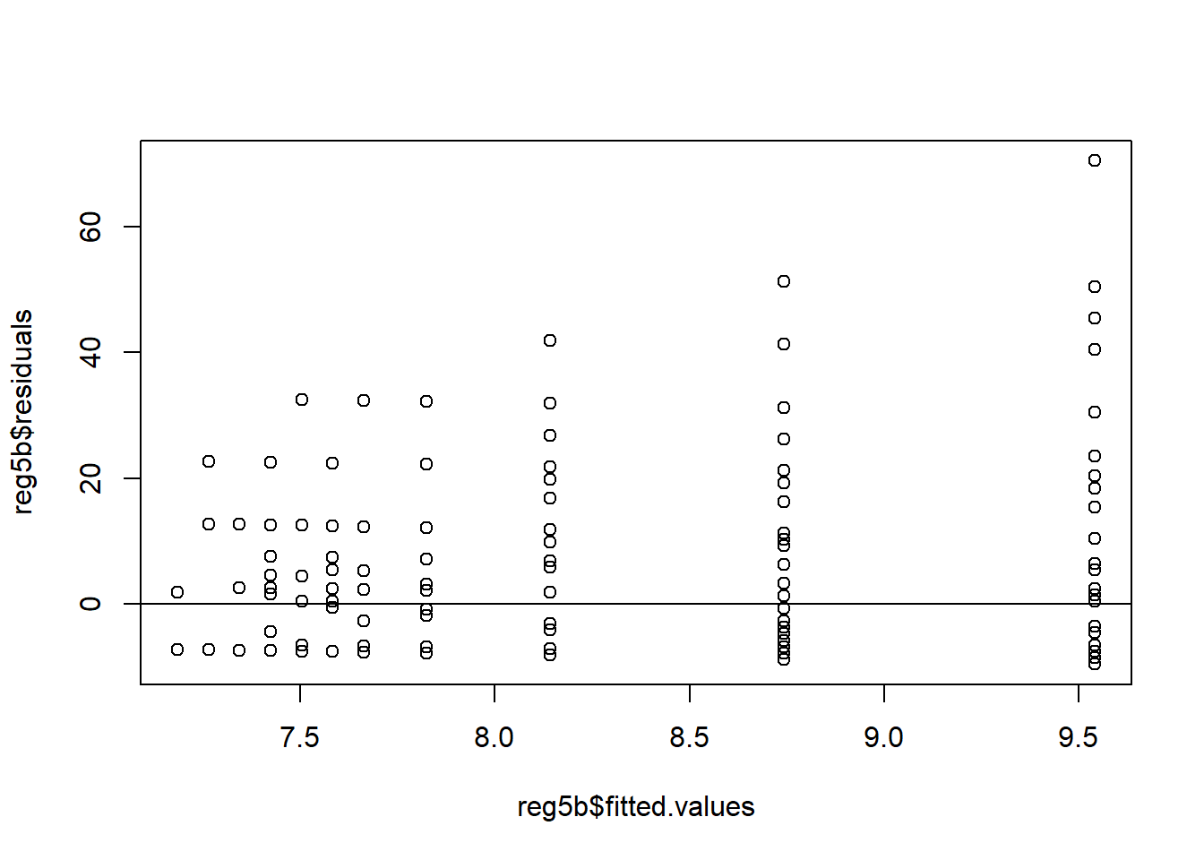
See how the shape of the residual plot looks a bit like a cone, with less spread on the left and a lot more spread on the right? This is evidence of heteroskedasticity. The residual plot doesn’t have to strictly be cone shaped for there to be heteroskedasticity, though that is the most common. Something that looks like a bow tie, or points scattered around a curved or sloped line would be considered heteroskedastic as well. Basically, any shape that isn’t a lot like that nice, neat rectangle from the vote1 data above exhibits heteroskedasticity.
The bad news is that, for the most part, academic economists simply assume that heteroskedasticity is always present. The good news is that there is a fairly simple and straightforward fix to it: calculating robust standard errors. In fact, nearly every regression in every academic journal will report robust standard errors as a matter of course. In R, we can get this from the lmtest library. If you haven’t already, install and load the sandwich library and use coeftest function with the vcovHC option.
coeftest(reg5b, vcovHC)##
## t test of coefficients:
##
## Estimate Std. Error t value Pr(>|t|)
## (Intercept) 7.1447e+00 9.9532e-01 7.1783 1.606e-12 ***
## income 7.9866e-05 4.9948e-05 1.5990 0.1102
## ---
## Signif. codes: 0 '***' 0.001 '**' 0.01 '*' 0.05 '.' 0.1 ' ' 1We can compare this result side-by-side with the original regression:
stargazer(reg5b, coeftest(reg5b, vcovHC), type = "text")##
## ===================================================
## Dependent variable:
## -------------------------------
## cigs
## OLS coefficient
## test
## (1) (2)
## ---------------------------------------------------
## income 0.0001 0.0001
## (0.0001) (0.00005)
##
## Constant 7.145*** 7.145***
## (1.128) (0.995)
##
## ---------------------------------------------------
## Observations 807
## R2 0.003
## Adjusted R2 0.002
## Residual Std. Error 13.711 (df = 805)
## F Statistic 2.286 (df = 1; 805)
## ===================================================
## Note: *p<0.1; **p<0.05; ***p<0.01It’s a bit tough to see here, but the coefficients didn’t change at all, and they shouldn’t. The only change is in the the standard errors (the numbers in the parentheses) underneath the coefficients. Because the standard errors change (they could go up or down!), the significance of the coefficients may change as well.
For example, let’s consider these regressions using the infmrt infant mortality data in the wooldridge package. This next bit of code estimates infant mortality, \(infmort\), as a function of the share of families receiving Aid to Families with Dependent Children (AFDC) and the number of physicians per capita. I then show those results side-by-side with the same regression corrected for heteroskedasticity.
reg5z <- lm(infmort ~ afdcper + physic, data = infmrt)
stargazer(reg5z, coeftest(reg5z, vcovHC), type = "text")
##
## ======================================================
## Dependent variable:
## ----------------------------------
## infmort
## OLS coefficient
## test
## (1) (2)
## ------------------------------------------------------
## afdcper 0.395*** 0.395***
## (0.139) (0.142)
##
## physic 0.008*** 0.008
## (0.003) (0.008)
##
## Constant 6.497*** 6.497***
## (0.601) (1.637)
##
## ------------------------------------------------------
## Observations 102
## R2 0.240
## Adjusted R2 0.225
## Residual Std. Error 1.813 (df = 99)
## F Statistic 15.672*** (df = 2; 99)
## ======================================================
## Note: *p<0.1; **p<0.05; ***p<0.01Again, compare the columns. The coefficients do not change, but the standard errors do. And, as stated above, this can have the effect of changing the significance of one or more of your coefficients; in this case, physicians per capita went from having a significant (at the 1% level!) relationship with infant mortality to having an insignificant relationship.
If a model is not heteroskedastic and doesn’t have autocorrelation, it is said to have spherical errors and the error terms are IID (Independent and Identically Distributed).
6.6 Assumption 6: No Independent Variable is a Perfect Linear Function of other Explanatory Variables.
This one is important and will probably create quite a few headaches for you when we get to regression with categorical independent variables in Chapter 7. Let’s introduce the concept quickly here though.
As discussed in a previous notebook, ordinary least squares works by attributing the variation in the dependent variable (Y) to the variation in your independent variables (the Xs). If you have more than one independent variable, OLS needs to figure out which independent variable to attribute the variation to. If you have two identical independent variables, R cannot distinguish one variable from the other when trying to apportion variation. If you attempt to estimate a model that contains independent variables that are perfectly correlated, R will attempt to thwart you. Typically, the way to proceed is to simply remove one of the offending variables.
So, let’s see what happens if I try to run a regression with the same variable twice:
reg6a <- lm(voteA ~ shareA + shareA, data = vote1)
stargazer(reg6a, type = "text")
##
## ===============================================
## Dependent variable:
## ---------------------------
## voteA
## -----------------------------------------------
## shareA 0.464***
## (0.015)
##
## Constant 26.812***
## (0.887)
##
## -----------------------------------------------
## Observations 173
## R2 0.856
## Adjusted R2 0.855
## Residual Std. Error 6.385 (df = 171)
## F Statistic 1,017.663*** (df = 1; 171)
## ===============================================
## Note: *p<0.1; **p<0.05; ***p<0.01Thwarted! R doesn’t even let me run this–note that shareA is only included in the table once. So let’s trick it into running a regression with two identical variables. I will display the results both with stargazer and summary, because stargazer will do its best to disguise my ineptitude here:
tempdata3 <- vote1
tempdata3$shareAclone <- tempdata3$shareA
reg6b <- lm(voteA ~ shareA + shareAclone, data = tempdata3)
stargazer(reg6b, type = "text")
##
## ===============================================
## Dependent variable:
## ---------------------------
## voteA
## -----------------------------------------------
## shareA 0.464***
## (0.015)
##
## shareAclone
##
##
## Constant 26.812***
## (0.887)
##
## -----------------------------------------------
## Observations 173
## R2 0.856
## Adjusted R2 0.855
## Residual Std. Error 6.385 (df = 171)
## F Statistic 1,017.663*** (df = 1; 171)
## ===============================================
## Note: *p<0.1; **p<0.05; ***p<0.01summary(reg6b)##
## Call:
## lm(formula = voteA ~ shareA + shareAclone, data = tempdata3)
##
## Residuals:
## Min 1Q Median 3Q Max
## -16.8919 -4.0660 -0.1682 3.4965 29.9772
##
## Coefficients: (1 not defined because of singularities)
## Estimate Std. Error t value Pr(>|t|)
## (Intercept) 26.81221 0.88721 30.22 <2e-16 ***
## shareA 0.46383 0.01454 31.90 <2e-16 ***
## shareAclone NA NA NA NA
## ---
## Signif. codes: 0 '***' 0.001 '**' 0.01 '*' 0.05 '.' 0.1 ' ' 1
##
## Residual standard error: 6.385 on 171 degrees of freedom
## Multiple R-squared: 0.8561, Adjusted R-squared: 0.8553
## F-statistic: 1018 on 1 and 171 DF, p-value: < 2.2e-16Now R is quite displeased with us. R simply dropped the shareAclone variable because it is impossible to run a regression with both shareA and shareAclone.
Let’s dig a little deeper into the linear function idea. Assume that you are running a regression with 3 independent variables, \(X_1\), \(X_2\), and \(X_3\).
\[\begin{equation} Y = \alpha + \beta_1 X_{1} + \beta_2 X_{2} +\beta_3 X_{3} +\epsilon_i \end{equation}\]
This assumption basically states that:
- \(X_1\), \(X_2\), and \(X_3\) are all different variables.
- \(X_1\) is not simply a rescaled version of \(X_2\) or \(X_3\). For example, If \(X_1\) is height in inches, \(X_2\) can’t be height in centimeters because then \(X_2 = 2.5X_1\)
- \(X_1\) cannot be reached with a linear combination of \(X_2\) and \(X_3\). So, if \(X_1\) is income, \(X_2\) is consumption, and \(X_3\) is savings, and thus \(X_1 = X_2 + X_3\), you can’t include all 3 variables in your equation. This is true of more compicated linear combinations as well; if \(X_1 = 23.1 + .2X_2 - 12.4X_3\), you couldn’t run that either.
This probably doesn’t seem like it would be an issue. However, this assumption trips up a lot of people who are new to regression, because they are not usually aware that there is another variable hidden in the regression, \(X_0\), which carries a value of 1 for every observation. This is technically what the \(\alpha\) is multiplied by. So in actuality, your regression model is
\[\begin{equation} Y = \alpha X_{0}+ \beta_1 X_{1} + \beta_2 X_{2} +\beta_3 X_{3} +\epsilon_i \end{equation}\]
Since \(X_{0}\) is 1, we don’t bother writing it out every time, but it is there. And so this means that \(X_1\), \(X_2\), and \(X_3\) cannot be constants, because otherwise you will violate this assumption.
Let’s see what happens when we include another constant in the voting model:
tempdata3$six <- 6
reg6c <- lm(voteA ~ shareA + six, data = tempdata3)
summary(reg6c)
##
## Call:
## lm(formula = voteA ~ shareA + six, data = tempdata3)
##
## Residuals:
## Min 1Q Median 3Q Max
## -16.8919 -4.0660 -0.1682 3.4965 29.9772
##
## Coefficients: (1 not defined because of singularities)
## Estimate Std. Error t value Pr(>|t|)
## (Intercept) 26.81221 0.88721 30.22 <2e-16 ***
## shareA 0.46383 0.01454 31.90 <2e-16 ***
## six NA NA NA NA
## ---
## Signif. codes: 0 '***' 0.001 '**' 0.01 '*' 0.05 '.' 0.1 ' ' 1
##
## Residual standard error: 6.385 on 171 degrees of freedom
## Multiple R-squared: 0.8561, Adjusted R-squared: 0.8553
## F-statistic: 1018 on 1 and 171 DF, p-value: < 2.2e-16R didn’t like the constant in the regression and just chucked it out. Why? Because the variable I called \(six\) is literally \(X_{0}+5\), which makes it a linear function of the intercept term!
Remember this lesson for when we start talking about dummy variable regressions in Chapter 7, it’s going to be important!
A related issue you might run into is multicollinearity, which is where you don’t have perfectly correlated independent variables but they are very, very close. If these correlations are high enough, they generally cause problems. Let’s see what happens when we run a regression with multicollinear independent variables.Here, I will use the voting data and create a new variable called shareArand which is the value of shareA plus a random number between -1 and 1.
set.seed(8675309)
tempdata4 <- tempdata3 %>%
    mutate(shareArand = shareA + runif(173, min = -1, max = 1))
cor(tempdata4$shareA, tempdata4$shareArand)
## [1] 0.9998562You can see that shareA and shareArand are very highly correlated. But they are not exactly the same, so we haven’t violated our assumption. What happens when I run this regression? Weird stuff:
reg6d <- lm(voteA ~ shareA + shareArand, data = tempdata4)
reg6e <- lm(voteA ~ shareArand, data = tempdata4)
stargazer(reg6a, reg6e, reg6d, type = "text")
##
## ==================================================================================================
## Dependent variable:
## ------------------------------------------------------------------------------
## voteA
## (1) (2) (3)
## --------------------------------------------------------------------------------------------------
## shareA 0.464*** -1.231
## (0.015) (0.850)
##
## shareArand 0.464*** 1.693**
## (0.014) (0.849)
##
## Constant 26.812*** 26.821*** 26.911***
## (0.887) (0.882) (0.881)
##
## --------------------------------------------------------------------------------------------------
## Observations 173 173 173
## R2 0.856 0.858 0.859
## Adjusted R2 0.855 0.857 0.858
## Residual Std. Error 6.385 (df = 171) 6.350 (df = 171) 6.330 (df = 170)
## F Statistic 1,017.663*** (df = 1; 171) 1,030.650*** (df = 1; 171) 519.686*** (df = 2; 170)
## ==================================================================================================
## Note: *p<0.1; **p<0.05; ***p<0.01Columns 1 and 2 have the original data and slightly adulterated data, respectively. Note that the results are very similar, though not identical. Now, Compare the model with the multicollinearity on the right with the original model on the left. The coefficients are huge in absolute value compared to column 1. One of the coefficients has the wrong sign.
Note that if you add the two \(\beta\)s in column 3 together, you get a number very close to the coefficient on shareA in column 1. This result is typical of models with multicollinearity.
Multicollinearity is a problem, but it is a very easy problem to fix. Just drop one of the collinear variables and the problem is solved.

6.7 Assumption 7: Normality of Error Terms
The last assumption of the regression model is that your error terms are normally distributed. Violating this assumption is not terrible, but if this assumption is violated it is often a sign that your models might be heavily influenced by outliers. An easy way to look for this is the Q-Q plot. Let’s look at a Q-Q plot of the voting regression:
reg7a <- lm(voteA ~ shareA, data = vote1)
qqnorm(reg7a$residuals)
qqline(reg7a$residuals)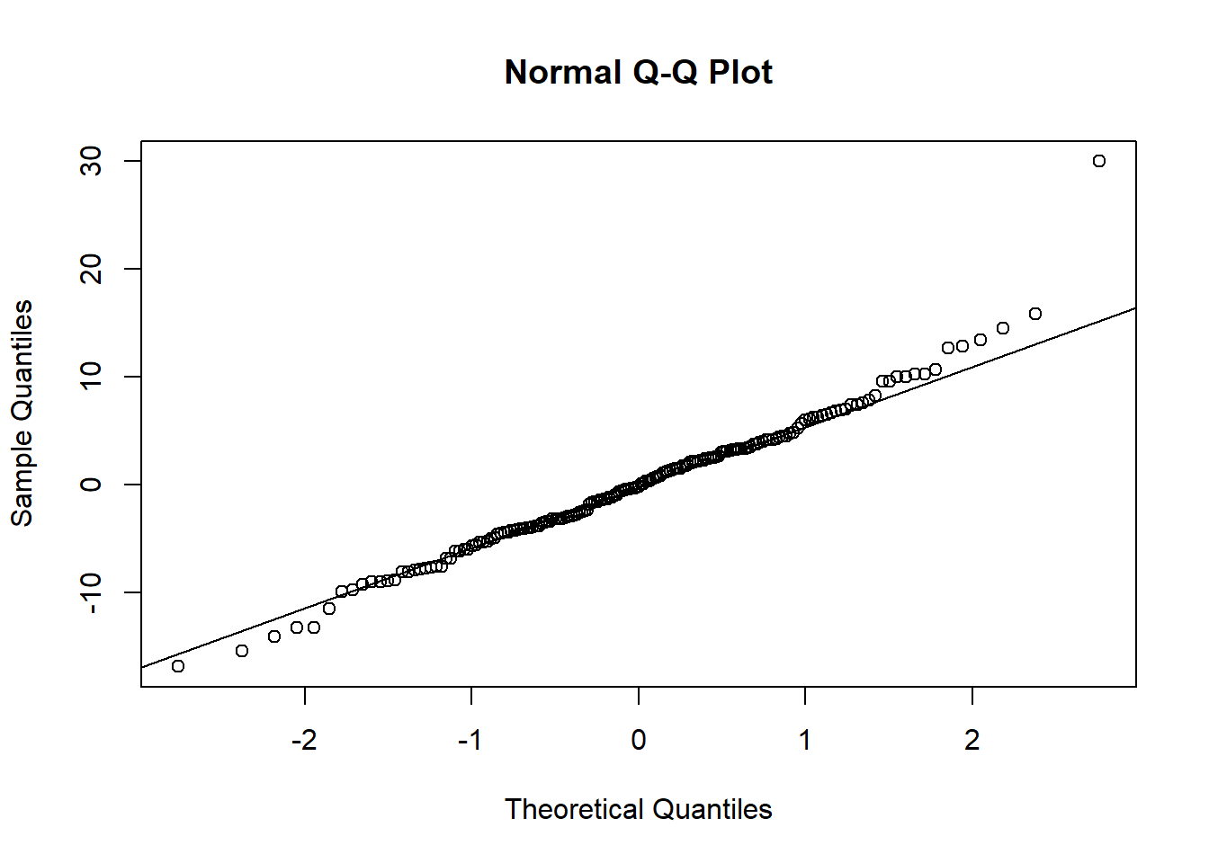
This Q-Q plot is pretty close to the line, indicating the residuals have pretty close to a normal distribution.
Let’s look at the Q-Q plot from the CEO salary regressions from up above:
qqnorm(reg1b$residuals)
qqline(reg1b$residuals)
Not quite as close to the line, but still not bad.
The Q-Q plot (and the residual plot from assumption 5) can be obtained another way; if you plot a regression object, you get 4 diagnostic plots, two of which are the ones we’ve looked at.
plot(reg7a)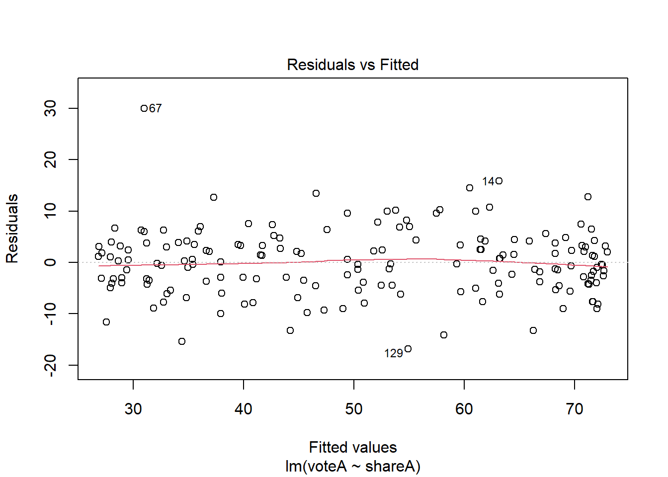
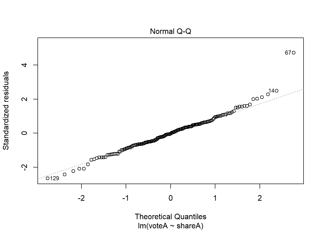
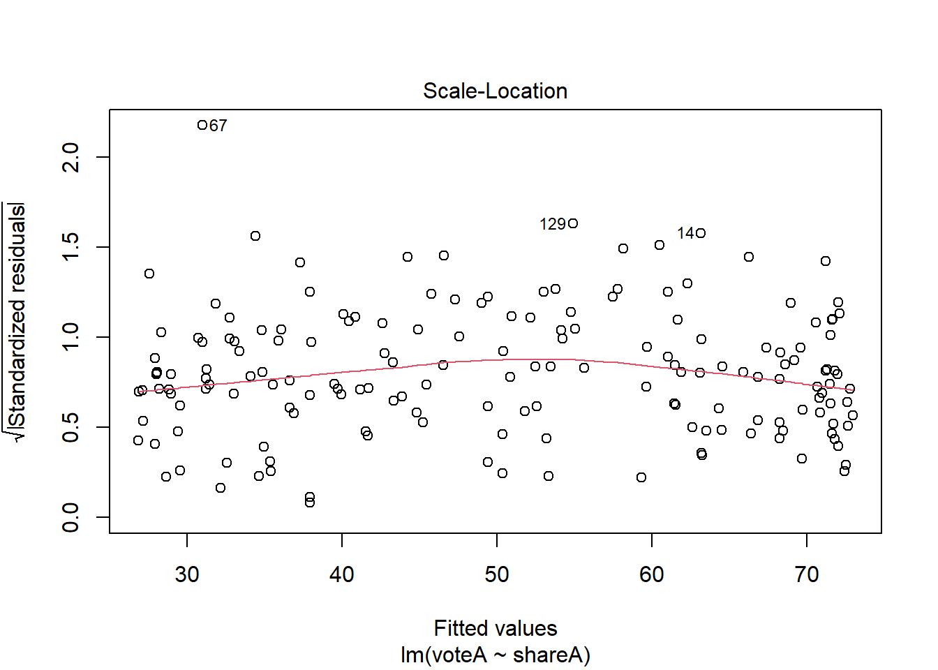
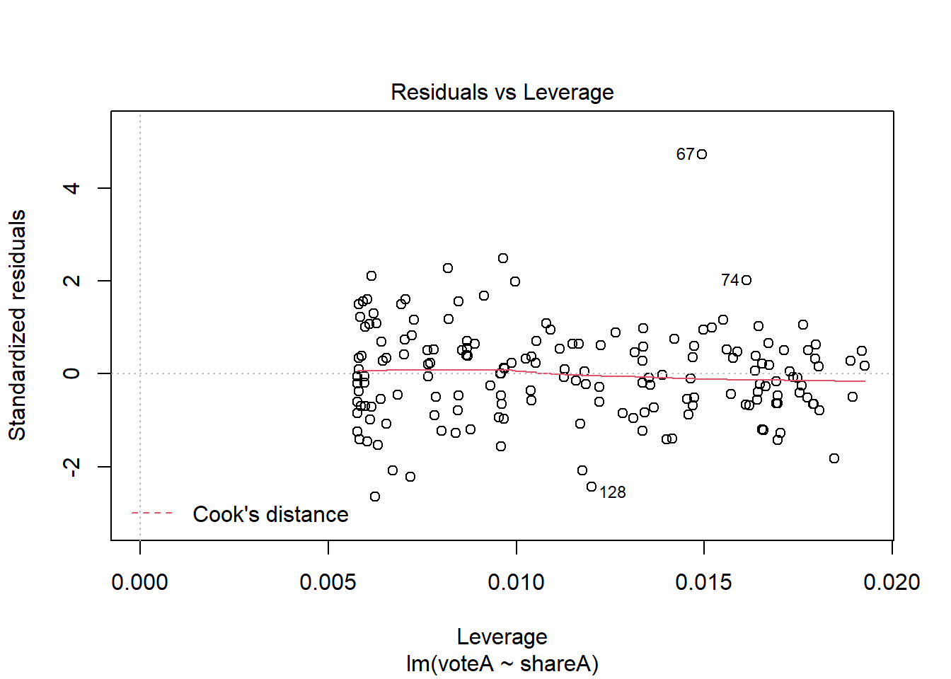
What do you do if your models are heavily influenced by outliers? Sometimes the right answer is to do nothing, especially if there are very few outliers relative to the size of the dataset. We’ve already discussed another approach in this chapter; using non-linear transformation. Beyond that, there are some very sophisticated approaches, like median regression (AKA Least Absolute Deviations) one can try, but these are well beyond the scope of this text.
6.8 Wrapping Up
This book is focused on learning the basic tools of econometrics; in line with that goal, I am totally aware that I did a considerable amount of handwaving (or straight up ignoring) with respect to some serious econometric issues. It is hard to draw the line in the sand between introductory econometrics and intermediate/advanced material, but that’s what I’m attempting to do here.
For those interested in pursuing careers in econometrics or business/data analytics, digging more deeply into these issues is essential. In the final chapter, Chapter 12, I list some suggested resources for those who wish to dig deeper into R or econometrics; many of the econometric suggestions in that section take much more comprehensive approaches into some of the issues presented here and would be excellent next steps for a reader interested in attaining a deeper understanding of econometrics.
Next, we will next turn to expanding the power of multiple regression modeling to include categorical independent variables and interaction effects.