Chapter 4 Inferential Statistics using R
This chapter provides a brief review of inferential statistics, including both basic univariate tests and some multivariate models, such as the t-test, ANOVA, and \(\chi ^2\). The other major family of multivariate models, regression, will be given a much more detailed treatment starting in Chapter 5, as regression modeling is the cornerstone of econometrics.
As always, let’s start by loading the relevant libraries and datasets into memory.
library(AER)
data(CPS1985)
attach(CPS1985)
library(wooldridge)
data(vote1)
attach(vote1)
data(k401k)
attach(k401k)
data(sleep)
data(affairs)
4.1 One-Sample t-test
Let’s start simple, with the 1-sample t-test. A 1-sample t-test is used to test a hypothesis about the mean of a specific data set.
We can illustrate the 1-sample t-test using the k401k data set from the wooldridge package. As always, ?k401k is a good way to get information about a data set.
?k401kThis data includes data on 1534 401k plans in the US. Suppose we are interested in the 401k match rate (i.e. for every dollar the 401k owner puts in, how much will the employer match with?), which is found in the \(mrate\) variable. To get a general overview of the data, we can look at the distribution of the contribution match rate with a simple histogram:
k401k %>% ggplot() +
    geom_histogram(aes(x = mrate), binwidth = .1)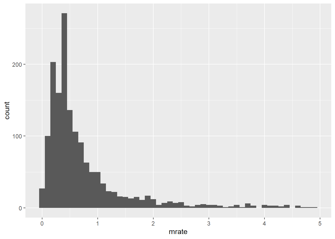
Just eyeballing the graph, it looks like the median and modal match rate is probably 50%, but there are some plans with some very generous match rates out there as this data is pretty heavily right-skewed.
Let’s say that an expert comes to you and tells you that the average (mean) match rate among 401k plans is 75%.
We can summarize the data and see that the mean in the data is 73.15%:
summary(mrate)## Min. 1st Qu. Median Mean 3rd Qu. Max.
## 0.0100 0.3000 0.4600 0.7315 0.8300 4.9100But is that far enough below 75% to dismiss the 75% claim? In other words, is it possible that the true mean actually is 75%, but by random chance our sample is not truly representative of the universe of 401k plans? Maybe our sample has disproportionately fewer 401ks with high match rates and more 401ks with low match rates than is true of the overall population? This is where a one-sample t-test comes in.
We should start by stating our Null and Alternative Hypotheses. In this case, our hypothesis is about our population mean (\(\mu\)), so we have:
- \(H_0\): \(\mu = .75\)
- \(H_1\): \(\mu \ne .75\)
In economics, it is common to use the confidence level of 0.95 (or p<0.05).

The t-test is executed with the t.test() function.
t.test(mrate, alternative = "two.sided", mu = .75, conf.level = 0.95)##
## One Sample t-test
##
## data: mrate
## t = -0.92887, df = 1533, p-value = 0.3531
## alternative hypothesis: true mean is not equal to 0.75
## 95 percent confidence interval:
## 0.6924718 0.7705530
## sample estimates:
## mean of x
## 0.7315124Here, we se see the results of the t-test. The results state that we do not have enough evidence to reject \(H_0\), the expert’s claim. Why not? There are quite a few things in the output that indicate that we should not reject \(H_0\):
- the p-value (\(p=0.3531\)) is not less than 0.05
- the confidence interval (.69 to 0.77) includes our hypothesized value of 0.75
- the t value (-0.929) is not in the rejection region (it would have to be less than -1.96–you can use the
qt()function to look up t-values)
Let’s say that this same expert tells you that the average participation rate, \(prate\), in 401k programs is over 90% This indicates a 1 sided test, where:
- \(H_0\): \(\mu \geq .9\)
- \(H_1\): \(\mu < .9\)
We can calculate a one-sided t-test for prate as follows:
t.test(prate, alternative = "less", mu = 90, conf.level = .95)##
## One Sample t-test
##
## data: prate
## t = -6.1786, df = 1533, p-value = 4.135e-10
## alternative hypothesis: true mean is less than 90
## 95 percent confidence interval:
## -Inf 88.06537
## sample estimates:
## mean of x
## 87.36291This suggests that we reject the null hypothesis, that the mean in the data set of 87.4 is far enough below 90 to say that the true mean is probably below 90. We see this in the results because:
- the p-value (\(p=4.135e-10\)) is definitely less than 0.05
- the confidence interval ($-$ to 88.1) does not include our hypothesized value of 90
- the t value (-6.18) is in the rejection region (it starts around -1.65)
It is often useful to store the results of a test in an object, for example:
test1 <- t.test(prate, alternative = "less", mu = 90, conf.level = .95)An object called test1 should be in your environment window.
To see what is in this object, see what its attributes() are:
attributes(test1)## $names
## [1] "statistic" "parameter" "p.value" "conf.int" "estimate"
## [6] "null.value" "stderr" "alternative" "method" "data.name"
##
## $class
## [1] "htest"Now, you can refer to these elements using the $.
test1$statistic## t
## -6.178623test1$estimate## mean of x
## 87.362914.2 Two-Sample t-test
The two-sample t-test is used to compare the means of two populations. Typically, you are looking at a situation where you have a numeric dependent variable that you think varies based on the value of some categorical independent variable that has two possible levels.
Let’s consider the CPS1985 data. Perhaps you think that union members have higher incomes than non-union members. Here, wage is your numeric dependent variable, union membership is your categorical independent variable with 2 levels (union member and non-union member), so a two-sample t-test is appropriate. First, let’s start by looking at the data with a boxplot():
CPS1985 %>% ggplot(aes(y = wage, x = union)) +
geom_boxplot()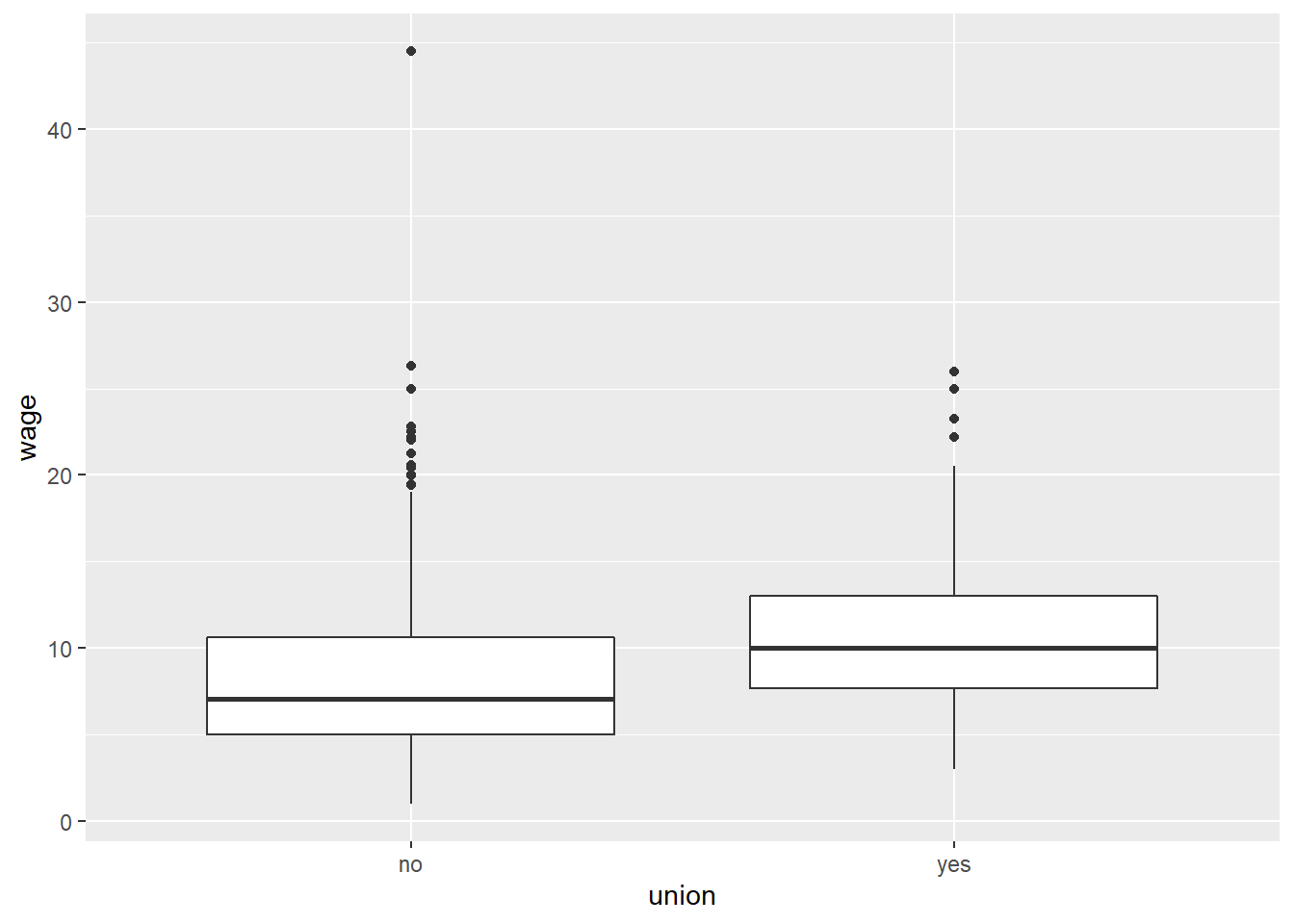 Again, we should start by stating our Null and Alternative Hypotheses. In this case, our hypothesis is about our population mean (mu), so we have:
- \(H_0\): \(\mu_{union} = \mu_{non-union}\)
- \(H_1\): \(\mu_{union} \ne \mu_{non-union}\)
Based on the graph, it looks like there may be a difference, but there are a lot of outliers so it’s tough to tell justby eyeballing it. Let’s do the statistical test using the same t.test() command as before. Here, we use the code wage ~ union. Again, the tilde ~ is the formula operator; when I see I tilde, in my head I say “is a function of” so I read wage ~ union to say that wage is a function of union membership.
Another way to think about the ~ operator is that it separates the dependent variable from the independent variable(s), with the syntax of Dependent Variable ~ Independent Variable(s). The dependent variable goes on the left, the independent variable on the right.
t.test(wage ~ union, mu = 0, alt = "two.sided", conf.level = .95)##
## Welch Two Sample t-test
##
## data: wage by union
## t = -4.1025, df = 153.69, p-value = 6.608e-05
## alternative hypothesis: true difference in means between group no and group yes is not equal to 0
## 95 percent confidence interval:
## -3.204407 -1.121386
## sample estimates:
## mean in group no mean in group yes
## 8.635228 10.798125The format of this code might be confusing at first glance. Why test mu=0? Technically, the test is that the difference of the means is equal to 0.
But that having been said, most of the arguments in this code are the default paramaters of the t.test() function anyhow. When you look at the help for t.test using ?t.test, it tells you what the default values are. The options mu = 0, alt = "two.sided", conf.level = .95 are all defaults, so this code can be simplified as:
t.test(wage ~ union)##
## Welch Two Sample t-test
##
## data: wage by union
## t = -4.1025, df = 153.69, p-value = 6.608e-05
## alternative hypothesis: true difference in means between group no and group yes is not equal to 0
## 95 percent confidence interval:
## -3.204407 -1.121386
## sample estimates:
## mean in group no mean in group yes
## 8.635228 10.798125Note that we get the same results. So why bother typing all the options? When you are learning R, typing all the options is a good way to learn the syntax.
Anyhow, what does this result tell us? We reject the null hypothesis!
- the p-value (p=6.608e-5) is less than 0.05
- the confidence interval (-3.2 to -1.1) does not include the value 0.
- the t value (-4.103) is in the rejection region (for this test we reject the null hypothesis if the absolute value of t is \(|t|>1.96\).
Let’s push a little farther with our two-sample t-tests. What if our research question is whether union membership affects wages, but only for males and only for those whose occupation is worker. How do we do this?
There are lots of ways–we could try to do it all using brackets to subset our data, or we could use dplyr to filter our data into a smaller dataset and do a simple t.test() as follows:
Option 1: bracketpalooza
t.test(wage[gender == "male" & occupation == "worker"] ~ union[gender == "male" & occupation == "worker"])##
## Welch Two Sample t-test
##
## data: wage[gender == "male" & occupation == "worker"] by union[gender == "male" & occupation == "worker"]
## t = -4.075, df = 70.168, p-value = 0.0001195
## alternative hypothesis: true difference in means between group no and group yes is not equal to 0
## 95 percent confidence interval:
## -4.828202 -1.655159
## sample estimates:
## mean in group no mean in group yes
## 8.03907 11.28075Option 2: Enter the Tidyverse
CPS1985 %>%
    filter(gender == "male") %>%
    filter(occupation == "worker") %>%
    t.test(wage ~ union, data = .)
##
## Welch Two Sample t-test
##
## data: wage by union
## t = -4.075, df = 70.168, p-value = 0.0001195
## alternative hypothesis: true difference in means between group no and group yes is not equal to 0
## 95 percent confidence interval:
## -4.828202 -1.655159
## sample estimates:
## mean in group no mean in group yes
## 8.03907 11.28075Both get to the same place. In my opinion, the tidyverse option is more elegant and easier to follow. The only tricky bit in there is the data = . part, which tells tidyverse to use the data I just filtered, but that’s just being fancy. I could have done:
tempdat <- CPS1985 %>%
    filter(gender == "male") %>%
    filter(occupation == "worker")
t.test(wage ~ union, data = tempdat)
##
## Welch Two Sample t-test
##
## data: wage by union
## t = -4.075, df = 70.168, p-value = 0.0001195
## alternative hypothesis: true difference in means between group no and group yes is not equal to 0
## 95 percent confidence interval:
## -4.828202 -1.655159
## sample estimates:
## mean in group no mean in group yes
## 8.03907 11.28075Which gets us to the same spot.
4.3 Wilcoxon / Mann-Whitney test
The Mann-Whitney U Test and the Wilcoxon Rank-Sum Test are similar tests. They can be used in place of the two-sample t-test in cases where the dataset is small or the data is non-normal. Let’s see if our wage data from the CPS1985 data is normal using a Quantile-Quantile plot (usually called a QQplot)
qqnorm(wage)
qqline(wage)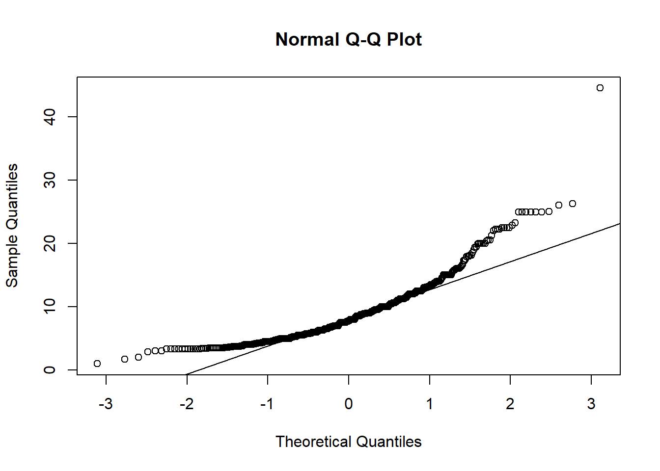
If the data were normal, they would lie (more or less) on the straight line. Because this Q-Q plot looks curved, it’s a decent indicator that our data is skewed.
To see what a normal Q-Q plot looks like, here is the Q-Q plot of the height variable in the trees dataset…it’s pretty darn close to normal!
qqnorm(trees$Height)
qqline(trees$Height)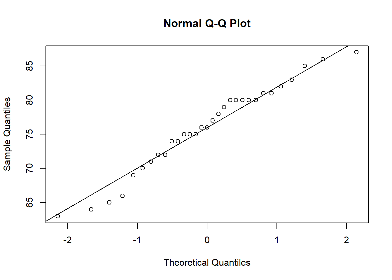
There’s actually a test to see if data is normally distributed called the Shapiro-Wilk test:
shapiro.test(wage)##
## Shapiro-Wilk normality test
##
## data: wage
## W = 0.8673, p-value < 2.2e-16shapiro.test(trees$Height)##
## Shapiro-Wilk normality test
##
## data: trees$Height
## W = 0.96545, p-value = 0.4034The null hypothesis is that the data is normal, so we reject the null for the wage data but do not for the trees data. This confirms that the distribution of the wage variable is non-normal while the distribution of the tree height variable probably is normal.
Anyhow, since it appears that our wage data may not be normal, perhaps a Wilcoxon test is in order. Rather than comparing the means, were are comparing the ranks of the data.
wilcox.test(wage ~ union)##
## Wilcoxon rank sum test with continuity correction
##
## data: wage by union
## W = 13780, p-value = 1.214e-07
## alternative hypothesis: true location shift is not equal to 0Here, the p-value is 1.2e-07, which is way less than .05, so again we reject the null hypothesis of these two groups being the same.
4.4 Paired t-Test
A paired t-test is used to compare 2 populations that are paired with each other. Often these are before-after type tests. The sleep data we loaded earlier shows the effect of 2 sleeping drugs given to 10 patients
sleep## extra group ID
## 1 0.7 1 1
## 2 -1.6 1 2
## 3 -0.2 1 3
## 4 -1.2 1 4
## 5 -0.1 1 5
## 6 3.4 1 6
## 7 3.7 1 7
## 8 0.8 1 8
## 9 0.0 1 9
## 10 2.0 1 10
## 11 1.9 2 1
## 12 0.8 2 2
## 13 1.1 2 3
## 14 0.1 2 4
## 15 -0.1 2 5
## 16 4.4 2 6
## 17 5.5 2 7
## 18 1.6 2 8
## 19 4.6 2 9
## 20 3.4 2 10Because the same group of people recieved both drugs, we can conduct a paired t-test here. This looks a lot like the 2 sample t-test we did earlier, with one extra argument:
t.test(extra ~ group, data = sleep, paired =TRUE)##
## Paired t-test
##
## data: extra by group
## t = -4.0621, df = 9, p-value = 0.002833
## alternative hypothesis: true difference in means is not equal to 0
## 95 percent confidence interval:
## -2.4598858 -0.7001142
## sample estimates:
## mean of the differences
## -1.584.5 ANOVA
ANOVA stands for Analysis of Variance and is a very common statistical technique in experimental sciences where one can run an experiment with a control group and multiple treatment groups. Though there are some notable exceptions, economics is not usually viewed as an experimental science. However, ANOVA is a special case of regression analysis, which is at the core of econometrics.
In many ways, ANOVA is just an amped-up 2-sample t-test; amped-up because you can have your dependent variable explained by more than 1 independent variable, and those independent variables can have more than two levels.
In the example we did above, we looked at the relationship between union membership and wages. Wages were the numeric dependent variable, and union membership was the 2-level (union or non-union) categorical variable.
Let’s calculate an ANOVA looking at the relationship between wages and occupation. We can start by looking at the data visually in a boxplot:
CPS1985 %>% ggplot(aes(x = occupation, y = wage)) +
    geom_boxplot(color = "blue4", fill = "cornflowerblue") +
    stat_boxplot(geom = "errorbar", width = 0.5)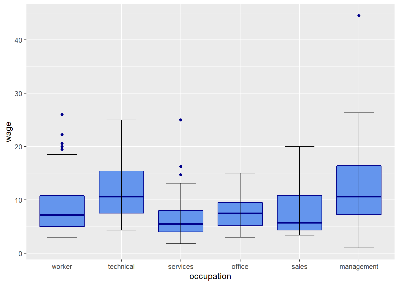
The Null hypothesis in ANOVA is that ALL of the means are the same…\(\mu_1 = \mu_2 = ... = \mu_k\). The alternative is that at least one is different from at least one other. It certainly looks like these means are different, but we can use ANOVA via the aov() command to test this.
aov(wage ~ occupation)## Call:
## aov(formula = wage ~ occupation)
##
## Terms:
## occupation Residuals
## Sum of Squares 2537.697 11539.001
## Deg. of Freedom 5 528
##
## Residual standard error: 4.674844
## Estimated effects may be unbalancedThe outupt of the aov() command doesn’t actually tell us much. We need to save this test result as an object and use the summary() command on that object.
anova1 <- aov(wage ~ occupation)
summary(anova1)
## Df Sum Sq Mean Sq F value Pr(>F)
## occupation 5 2538 507.5 23.22 <2e-16 ***
## Residuals 528 11539 21.9
## ---
## Signif. codes: 0 '***' 0.001 '**' 0.01 '*' 0.05 '.' 0.1 ' ' 1This table tells us whether or not we reject the null hypothesis…the Pr(>F) is our p-value, and that is way less than 0.05. so we reject the null hypothesis that all the group means are the same and accept the alternative hypothesis that at least one is different from the rest.
If we want to know which means are different, we can run the Tukey-Kremer test. To do this, we simply put our anova object into the TukeyHSD() function.
TukeyHSD(anova1)## Tukey multiple comparisons of means
## 95% family-wise confidence level
##
## Fit: aov(formula = wage ~ occupation)
##
## $occupation
## diff lwr upr p adj
## technical-worker 3.5209542 1.833122 5.20878674 0.0000001
## services-worker -1.8890045 -3.705623 -0.07238631 0.0361288
## office-worker -1.0038970 -2.732830 0.72503588 0.5584749
## sales-worker -0.8338428 -3.252714 1.58502882 0.9223496
## management-worker 4.2775256 2.180694 6.37435762 0.0000001
## services-technical -5.4099587 -7.373822 -3.44609529 0.0000000
## office-technical -4.5248513 -6.407898 -2.64180401 0.0000000
## sales-technical -4.3547970 -6.886120 -1.82347368 0.0000170
## management-technical 0.7565714 -1.469044 2.98218646 0.9265714
## office-services 0.8851074 -1.114190 2.88440478 0.8032931
## sales-services 1.0551617 -1.563792 3.67411581 0.8589942
## management-services 6.1665301 3.841732 8.49132800 0.0000000
## sales-office 0.1700543 -2.388857 2.72896576 0.9999657
## management-office 5.2814227 3.024479 7.53836588 0.0000000
## management-sales 5.1113684 2.290815 7.93192217 0.0000046This shows the confidence intervals and p-values for all of the pairwise comparisons–since there are 6 levels of the occupation variable, there are 6*5/2=15 different combinations to examine! We can display this visually by plotting the Tukey results:
plot(TukeyHSD(anova1))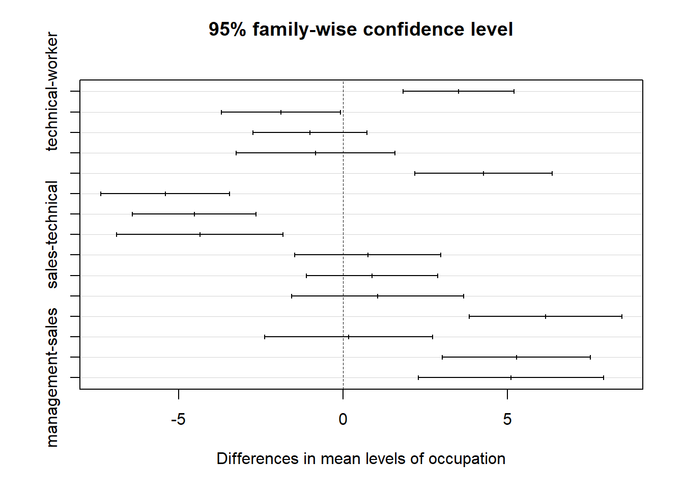
Ugh this is unreadable. Let’s try that again, some minor edits for readability:
par(mar = c(3,10,3,3))
plot(TukeyHSD(anova1), las = 1, cex.axis = .75)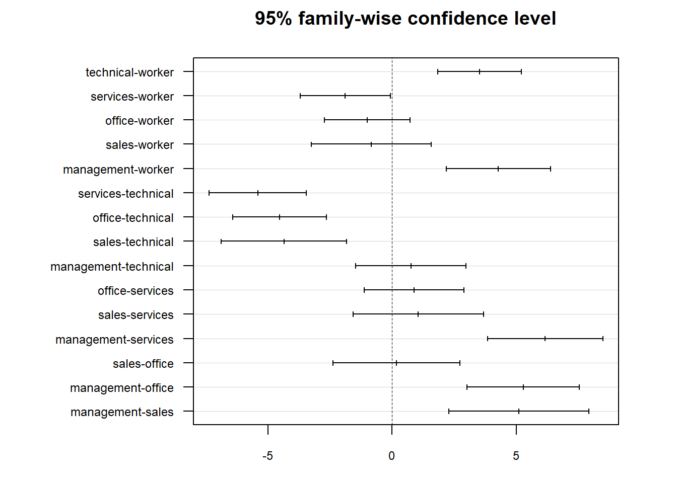
Any combination where 0 is not included in the confidence interval is considered to be a significant difference! It looks like there are quite a few of them.
The previous example is what is referred to as a 1-way ANOVA; 1-way refers to the fact that there is exactly one independent variable. In this case, that variable is occupation. ANOVA can include more than 1 independent variable in a version called 2-way ANOVA.
2-way ANOVA is more complex and allows us to have multiple independent categorical variables. Here, let’s look at wages as our dependent variable but have 2 categorical independent variables: gender and marital status.
This particular ANOVA has 3 null hypotheses:
- There is no difference in wages between men and women
- There is no difference in wages between married and unmarried individuals
- There is no interaction between gender and marital status.
Interaction is an complex idea. It is related to the idea in probability regarding independence. Here, an interaction effect would imply that either:
- The effect of gender on wages varies depends on whether or not the person is married or unmarried, or equivalently,
- The effect of marital status on wages depends on whether or not the person is a man or a woman.
Let’s take a look at this data graphically using a graph from the previous chapter:
CPS1985 %>% ggplot(aes(x = married, y = wage, fill = gender)) +
    geom_boxplot() +
    theme_classic() +
    labs(title = "Does Marriage Influnce the Gender Wage Gap?",
         subtitle = "1985 CPS data",
         x = "Marital Status",
         y = "Wages",
         fill = "",
         caption = "@mattdobra") +
    scale_fill_manual(values= c("deepskyblue4", "darksalmon")) +
    theme(legend.position = "bottom",
          legend.direction = "horizontal",
          axis.ticks.x = element_blank()) +
    scale_x_discrete(labels = c("no" = "Unmarried", "yes" = "Married"))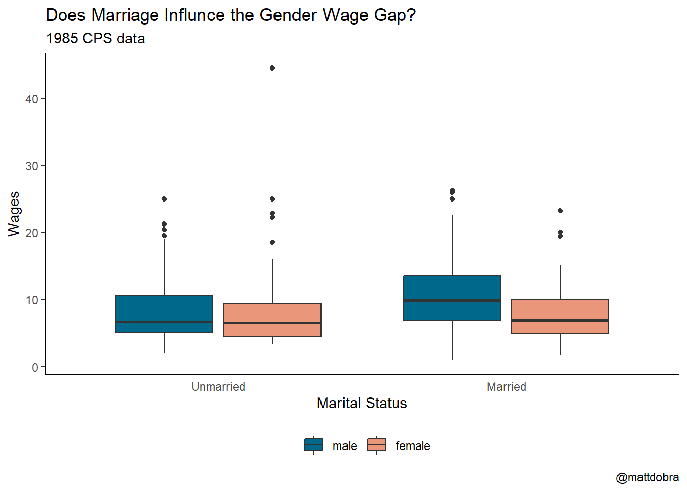
Let’s run this ANOVA and see what the results are:
anova2<-aov(wage ~ gender*married)
summary(anova2)
## Df Sum Sq Mean Sq F value Pr(>F)
## gender 1 594 593.7 24.118 1.21e-06 ***
## married 1 149 149.0 6.054 0.01420 *
## gender:married 1 287 286.8 11.652 0.00069 ***
## Residuals 530 13047 24.6
## ---
## Signif. codes: 0 '***' 0.001 '**' 0.01 '*' 0.05 '.' 0.1 ' ' 1We can reject all 3 null hypotheses at the 5% level. We can dig deeper into the results by looking at the Tukey-Kremer test:
TukeyHSD(anova2)## Tukey multiple comparisons of means
## 95% family-wise confidence level
##
## Fit: aov(formula = wage ~ gender * married)
##
## $gender
## diff lwr upr p adj
## female-male -2.116056 -2.962502 -1.269611 1.2e-06
##
## $married
## diff lwr upr p adj
## yes-no 1.111544 0.2240042 1.999084 0.0142019
##
## $`gender:married`
## diff lwr upr p adj
## female:no-male:no -0.09511392 -1.9895353 1.7993075 0.9992257
## male:yes-male:no 2.52131135 0.9437846 4.0988381 0.0002573
## female:yes-male:no -0.67098704 -2.2921516 0.9501775 0.7099932
## male:yes-female:no 2.61642528 0.9312927 4.3015579 0.0004171
## female:yes-female:no -0.57587312 -2.3019252 1.1501790 0.8255032
## female:yes-male:yes -3.19229840 -4.5630697 -1.8215271 0.0000000The bottom panel examines the interaction effects, and is pretty interesting.
- The difference in wages between unmarried men and unmarried women is insignificant.
- The difference in wages between married females and unmarried females is insignificant.
But:
- The difference between married women and married men is significant
- The difference between married men and unmarried men is significant
Interpreting results like this add nuance to the issue of the gender wage gap.
This is enough ANOVA for here. Econometrics typically focuses on regression analysis, not ANOVA. And, for what its worth, ANOVA is just a very special case of regression analysis anyhow.
4.6 Chi-Square
The Chi-Square test (sometimes stylized as \(\chi^2\)) looks at relationships between 2 (or more) categorical variables. Whereas ANOVA had categorical independent variables with numeric dependent variables, Chi-Square has both categorial independent and dependent variables. Let’s look at the affairs dataset from the AER package. This data is from a 1978 paper that looks into the prevalence of extramarital affairs. We might ask the question whether or not there is a relationship between extramarital affairs and whether or not a married couple has kids.
Let’s start by making a cross tabulation of couples with kids and couples where an affair is occurring. It is easiest to use dplyr to create a new data frame that only has the 2 variables of interest.
affair2 <- affairs %>% select(c(affair, kids))
table(affair2)
## kids
## affair 0 1
## 0 144 307
## 1 27 123On a percentage basis, it looks like affairs are more prevalent among couples with kids. Maybe this is more clear with a graph:
affairs %>%
    ggplot(aes(x = as.factor(kids), fill = as.factor(affair))) +
    geom_bar(position = "fill") +
    scale_fill_viridis_d() +
    labs(y = "")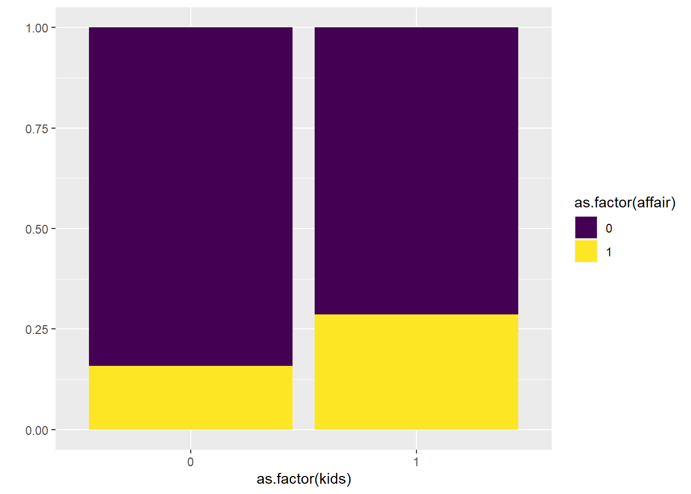
Is this difference big enough to be statistically significant? This is where we call in the Chi-Square test:
chisq.test(affairs$kids, affairs$affair)##
## Pearson's Chi-squared test with Yates' continuity correction
##
## data: affairs$kids and affairs$affair
## X-squared = 10.055, df = 1, p-value = 0.00152The p-value is less than .05, so it appears that there is a statistically significant difference in the rate of affairs between couples with kids from those without kids.
4.7 Wrapping Up
The metnods seen in this chapter are not frequently used in either economics or data science. Because these methods require that all of the independent variables used be categorical, their primary value lies in the world of experimental research.
It is very frequently the case that we want to examine independent variables that are numeric. This poses a problem for models like ANOVA and Chi-Square, because in order to use a numeric independent variable in one of these models, we need to create a set of ad hoc categories to fit our numeric data into, and in the process losing much of the variation (and thus information) in the data. None of this is ideal.
There is a modeling technique that allows us to use both categorical and numeric independent variables: regression analysis. Regression forms the basic building block of econometrics and of data science, and is the focus of the irest of this text.
4.8 End of Chapter Exercises
ANOVA:
Use the famous
datasets:irisdata to see if any of the 4 measures of iris size (\(Sepal.Length\),\(Sepal.Width\),\(Petal.Length\),\(Petal.Width\)) varies by iris \(Species\). Create boxplots and analyze each of the flower characteristics with one-way ANOVA, and if any of your ANOVAs indicate that you should reject the null hypothesis, follow up with Tukey-Kramer tests to identify which pairs are statistically different.Use the
datasets:mtcarsdata to see if size of an engine as measured in number of cylinders (\(cyl\)) influences fuel efficiency (\(mpg\)), power (\(hp\)), or speed (\(qsec\)). Important: Make sure you force R to treat the cylinder variable as a factor, not a number! Create boxplots and analyze each of the performance characteristics with one-way ANOVA, and if any of your ANOVAs indicate that you should reject the null hypothesis, follow up with Tukey-Kramer tests to identify which pairs are statistically different.