Recursion and Interest

Simple and Compound Interest

Let’s relate the chessboard problem to that of simple and compound interest. We will use the definitions from wikipedia for these as a starting place.

Simple Interest: is calculated only on the principal amount, or on that portion of the principal amount that remains. It excludes the effect of compounding. Simple interest can be applied over a time period other than a year, e.g. every month.
Compound Interest: Compound interest includes interest earned on the interest which was previously accumulated.

For example, let us suppose that money is deposited in an interest-bearing account at a bank. Let’s imagine this account returns an annual interest rate of 2.9% in simple interest. If this were compounded monthly, this would mean that we have a monthly rate of approximately .24%.

\[\text{monthly rate} = \displaystyle \frac{0.029}{12}\]

Each month we apply this interest applied to the initial deposit. If we deposit $500 at this interest rate, we would earn $500 \times 0.0024$ each month. We can use R to perform these calculations and then automate the addition with a for loop to simulate two years of interest.

rate <- 0.029/12
simple_interest <- 500
interest <- simple_interest * rate
for(i in 1:24){
    simple_interest[i+1] <- simple_interest[i] + interest
}
month <- seq(length(simple_interest))
earnings <- data.frame(month, simple_interest)
kable(head(earnings))

month	simple_interest
1	500.0000
2	501.2083
3	502.4167
4	503.6250
5	504.8333
6	506.0417

Now we can plot the results using ggplot2.

ggplot(earnings, aes(month, simple_interest)) +
  geom_point() +
  geom_line() +
  theme_minimal() +
  labs(title = "Simple interest over 24 months", x = "month", y = "total in account")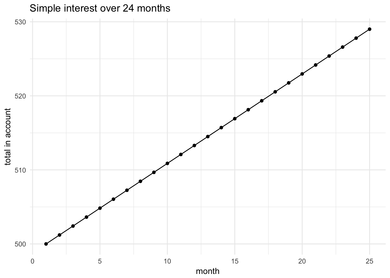

For compound interest, we want to repeatedly apply the interest rate to the amount of money in the account. For example, in month two, we would have $500 \times 0.0024 + 500$ in the account. Rather than adding the $500 \times 0.0024$ again, as we would with simple interest, we apply the interest to dollar amount in the account. This equates to using a for loop to repeatedly multiply the previous terms by the monthly interest rate. We create another dataframe and plot to represent the situation.

rate <- 0.029/12
compound_interest <- 500
for(i in 1:24){
    compound_interest[i+1] <- compound_interest[i] *rate + compound_interest[i]
}
month <- seq(length(compound_interest))
earnings_compound <- data.frame(month, compound_interest)
kable(head(earnings_compound))

month	compound_interest
1	500.0000
2	501.2083
3	502.4196
4	503.6338
5	504.8509
6	506.0709

We plot these results in a similar manner as the simple interest example.

ggplot(earnings_compound, aes(month, compound_interest)) +
  geom_point() +
  geom_line() +
  theme_minimal() +
  labs(title = "Compound interest over 24 months", x = "month", y = "Total in account")

Further, we can combine these dataframes using the inner_join function which will merge the dataframes by the common month column as follows.

library(tidyverse)

## Loading tidyverse: tibble
## Loading tidyverse: tidyr
## Loading tidyverse: readr
## Loading tidyverse: purrr
## Loading tidyverse: dplyr

## Conflicts with tidy packages ----------------------------------------------

## filter(): dplyr, stats
## lag():    dplyr, stats

compare <- inner_join(earnings, earnings_compound, by = "month")
kable(head(compare))

month	simple_interest	compound_interest
1	500.0000	500.0000
2	501.2083	501.2083
3	502.4167	502.4196
4	503.6250	503.6338
5	504.8333	504.8509
6	506.0417	506.0709

In order to use ggplot2 to plot these, we will further manipulate the table so that we have a column that associates the data with the label from the columns. We will do this with the melt function. Here, we will melt the “month”. Doing so produces a table with three columns, the first containing the months, the second the variable, and the third the value of the account depending on the variable. We will show the final amounts using a simple pipe.

library(reshape)

## 
## Attaching package: 'reshape'

## The following object is masked from 'package:dplyr':
## 
##     rename

## The following objects are masked from 'package:tidyr':
## 
##     expand, smiths

compare <- melt(compare, "month")
compare_end <- compare %>%
                  filter(month == 24)
kable(head(compare_end))

month	variable	value
24	simple_interest	527.7917
24	compound_interest	528.5431

Seems that the compound interest outperforms the simple interest. Per usual, we can plot this with ggplot.

ggplot(compare, aes(month, value), variable) +
    geom_line(aes(color = variable),  alpha = 0.7) +
    theme_minimal() +
    labs(title = "Simple vs. Compound Interest", subtitle = "24 Months at 2.9% Interest Compounded Monthly")