Functions and Static Representations

Mathematical Functions. As the Eames video begins, functions are proposed as invisible connections between two or more ‘things’. It’s important to note the mystical nature of this object. When we use functions to represent things, we are supposing a connection and usually a behavior for this connection.

The example of the candle from the video can be easily seen to connect to our last recursive definition. We are also able to define these with single formulas. For example, we could have the relationship:

\[\text{height of candle(hour) = initial candle height - one unit} \times \text{hour}\]

We would abbreviate this with something like

\[h(t) = 12 - t\]

Where h(t) is the height at some time t. We can use R to build functions easily as well. The code below deomonstrates how to write the function above in R.

h <- function(t){
        12 - t
}

Then, we can input some time and get back the height as follows.

h(3)

## [1] 9

If we want to plot this function over the first 12 hours, we simply need to define a list of input values. Below, the plot displays the function evaluated at each hour.

t <- seq(1:12)
plot(t, h(t))

Again, we will want to put this information in a table and use ggplot2 to visualize functions. Below, we create the dataframe and plot the function \(h\).

ht <- data.frame(t, h(t))
ggplot(ht, aes(t, h(t))) +
    geom_line() +
    theme_minimal() +
    labs(title = "Height of the Candle Versus Time", x = "Time in Hours", y = "Height in cm")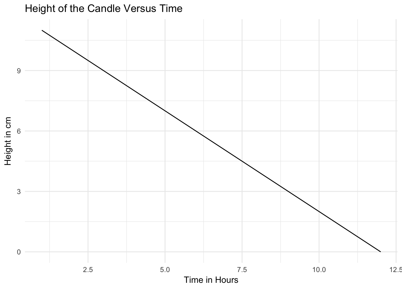

Simple and Compound Interest Closed Form

The formulas for Simple and Compound interest can be gleaned from the recursive form.

Simple Interest: Initial investment of P, interest rate r per frequency of compounding n, and number of time periods t.

\[S(t) = P + P \times \frac{r}{n} \times t \quad \text{or} \quad S(t) = P + P \times i \times t\]

Compount Interest: Same variables

\[C(t) = P(1 + \frac{r}{n})^t \quad \text{or} \quad C(t) = P(1 + i)^t\]

We can easily define functions that take as inputs the initial investment amount, the rate, and the time as follows.

s_int <- function(P, r, n, t){
                                P + P * (r/n) *t
}
c_int <- function(P, r, n, t){
                      P *(1 +(r/n))^t
}
t <- seq(1:36)

Now we can examine two investments using these functions over the time of 36 months.

S <- s_int(400, 0.039, 12, t)
C <- c_int(400, 0.039, 12, t)
ints <- data.frame(t, S, C)
kable(head(ints))

t	S	C
1	401.3	401.3000
2	402.6	402.6042
3	403.9	403.9127
4	405.2	405.2254
5	406.5	406.5424
6	407.8	407.8637

Finally, we melt the frame and plot it.

library(reshape)
library(ggplot2)
int_gg <- melt(ints, "t")
ggplot(int_gg, aes(t, value)) +
    geom_line(aes(color = variable)) +
    theme_minimal() +
    labs(title = "Graph of Simple versus Compound Interest as Functions", x = "Months", y = "Value")