Index Values

The problem of comparing change in money over time also involves understanding different approaches to understanding change. Just as simple and compound interest represent different types of change, we have different ways of understanding change between absolute change and relative change. Let’s take the example of the Cost of Education.(COMAP CPI INF) I’ve provided a small excel file with the data that we can read in with the readxl library’s read_excel function.

library(readxl)
library(knitr)
ed <- read_excel("cost_of_education.xlsx")
kable(head(ed), format = "html", caption = "Cost of Education over Time")

Table 2: Cost of Education over Time

Year	Tution	Annual Course Fees	Students with Fees	Textbook Cost per Course	Number of Courses	Supplies	Total
1986–87	5900	130	32	25	10.4	96	6297.6
1987–88	6450	130	29	27	10.5	98	6869.2
1988–89	7000	130	26	28	10.5	101	7428.8
1989–90	7650	140	28	31	10.6	104	8121.8
1990–91	8625	140	27	33	10.5	107	9116.3
1991–92	9450	150	25	35	10.4	110	9961.5

We can ask whether the change in Number of Courses was greater from 1990 to 1991 or 1987 to 1988. Absolute Change would be the absolute difference between the values found by subtracting them. We are interested in the relative change however, and want to know the percent change from year to year. For this example, we have the following percent change in classes:

\[\text{1990 to 1991} = \displaystyle \frac{107 - 104}{104} = 0.288\]

\[\text{1987 to 1988} = \displaystyle \frac{98 - 96}{96} = 0.208\]

\(~\)

To get an index number, divide the An index number provides a base index as a starting place and describes the percent change against this. For example, we would create an Education Cost Index from our data based on the 86 - 87 school year.

\[\frac{\text{Cost in Year XX}}{\text{Cost in 86-87}} = \frac{\text{Year XX Index}}{\text{86-87 Index}}\]

\[\text{Year XX Index} = 100 \times \frac{\text{Cost in Year XX}}{\text{Cost in 86-87}}\]

Let’s add a column to our dataframe that contains this information. We use the formula above to accomplish this. The following line of code adds a new column to our datafram titled “Index”. We note the call to ed[[1, "Total"]] with two brackets. This returns the value instead of a dataframe that we would get with single brackets.

\(~\)

ed["Index"]  <- 100*ed["Total"]/ed[[1, "Total"]]
kable(head(ed))

Year	Tution	Annual Course Fees	Students with Fees	Textbook Cost per Course	Number of Courses	Supplies	Total	Index
1986–87	5900	130	32	25	10.4	96	6297.6	100.0000
1987–88	6450	130	29	27	10.5	98	6869.2	109.0765
1988–89	7000	130	26	28	10.5	101	7428.8	117.9624
1989–90	7650	140	28	31	10.6	104	8121.8	128.9666
1990–91	8625	140	27	33	10.5	107	9116.3	144.7583
1991–92	9450	150	25	35	10.4	110	9961.5	158.1793

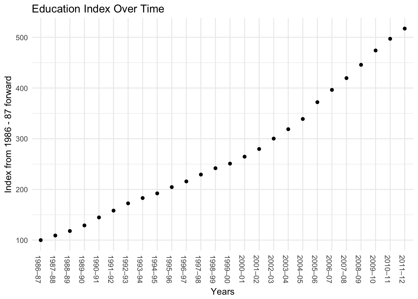
Finally, we can plot this index over time with ggplot.

ggplot(ed, aes(Year, Index)) +
    geom_point() +
    geom_line() +
    theme_minimal() +
    labs(title = "Education Index Over Time", x = "Years", y = "Index from 1986 - 87 forward") +
    theme(axis.text.x=element_text(angle = -90, hjust = 0))

## geom_path: Each group consists of only one observation. Do you need to
## adjust the group aesthetic?