16 Expected Values of Linear Combinations of Random Variables

16.1 Linear rescaling

If $X$ is a random variable and $a, b$ are non-random constants then

\[\begin{align*} \text{E}(aX + b) & = a\text{E}(X) + b\\ \text{SD}(aX + b) & = |a|\text{SD}(X)\\ \text{Var}(aX + b) & = a^2\text{Var}(X) \end{align*}\]

16.2 Linearity of expected value

Example 16.1

Refer to the tables and plots in Example 5.29 here. Each scenario contains SAT Math ($X$) and Reading ($Y$) scores for 10 hypothetical students, along with the total score ($T = X + Y$) and the difference between the Math and Reading scores ($D = X - Y$, negative values indicate lower Math than Reading scores). Note that the 10 $X$ values are the same in each scenario, and the 10 $Y$ values are the same in each scenario, but the $(X, Y)$ values are paired in different ways: the correlation is 0.78 in scenario 1, -0.02 in scenario 2, and -0.94 in scenario 3.

What is the mean of $T = X + Y$ in each scenario? How does it relate to the means of $X$ and $Y$? Does the correlation affect the mean of $T = X + Y$?
What is the mean of $D = X - Y$ in each scenario? How does it relate to the means of $X$ and $Y$? Does the correlation affect the mean of $D = X - Y$?

Linearity of expected value. For any two random variables $X$ and $Y$, \[\begin{align*} \text{E}(X + Y) & = \text{E}(X) + \text{E}(Y) \end{align*}\]
That is, the expected value of the sum is the sum of expected values, regardless of how the random variables are related.
Therefore, you only need to know the marginal distributions of $X$ and $Y$ to find the expected value of their sum. (But keep in mind that the distribution of $X+Y$ will depend on the joint distribution of $X$ and $Y$.)
Whether in the short run or the long run, \[\begin{align*} \text{Average of $X + Y$ } & = \text{Average of $X$} + \text{Average of $Y$} \end{align*}\] regardless of the joint distribution of $X$ and $Y$.
A linear combination of two random variables $X$ and $Y$ is of the form $aX + bY$ where $a$ and $b$ are non-random constants. Combining properties of linear rescaling with linearity of expected value yields the expected value of a linear combination. \[ \text{E}(aX + bY) = a\text{E}(X)+b\text{E}(Y) \]
Linearity of expected value extends naturally to more than two random variables.

16.3 Variance of linear combinations of random variables

Example 16.2

Recall Example 16.1.

In which of the three scenarios is $\text{Var}(X + Y)$ the largest? Can you explain why?
In which of the three scenarios is $\text{Var}(X + Y)$ the smallest? Can you explain why?
In which scenario is $\text{Var}(X + Y)$ roughly equal to the sum of $\text{Var}(X)$ and $\text{Var}(Y)$?
In which of the three scenarios is $\text{Var}(X - Y)$ the largest? Can you explain why?
In which of the three scenarios is $\text{Var}(X - Y)$ the smallest? Can you explain why?
In which scenario is $\text{Var}(X - Y)$ roughly equal to the sum of $\text{Var}(X)$ and $\text{Var}(Y)$?

Variance of sums and differences of random variables. \[\begin{align*} \text{Var}(X + Y) & = \text{Var}(X) + \text{Var}(Y) + 2\text{Cov}(X, Y)\\ \text{Var}(X - Y) & = \text{Var}(X) + \text{Var}(Y) - 2\text{Cov}(X, Y) \end{align*}\]

Example 16.3

Assume that SAT Math ($X$) and Reading ($Y$) scores follow a Bivariate Normal distribution, Math scores have mean 527 and standard deviation 107, and Reading scores have mean 533 and standard deviation 100. Compute $\text{Var}(X + Y)$ and $\text{SD}(X+Y)$ for each of the following correlations.

$\text{Corr}(X, Y) = 0.77$
$\text{Corr}(X, Y) = 0.40$
$\text{Corr}(X, Y) = 0$
$\text{Corr}(X, Y) = -0.77$

Example 16.4

Continuing the previous example. Compute $\text{Var}(X - Y)$ and $\text{SD}(X-Y)$ for each of the following correlations.

$\text{Corr}(X, Y) = 0.77$
$\text{Corr}(X, Y) = 0.40$
$\text{Corr}(X, Y) = 0$
$\text{Corr}(X, Y) = -0.77$

The variance of the sum is the sum of the variances if and only if $X$ and $Y$ are uncorrelated. \[\begin{align*} \text{Var}(X+Y) & = \text{Var}(X) + \text{Var}(Y)\qquad \text{if $X, Y$ are uncorrelated}\\ \text{Var}(X-Y) & = \text{Var}(X) + \text{Var}(Y)\qquad \text{if $X, Y$ are uncorrelated} \end{align*}\]
The variance of the difference of uncorrelated random variables is the sum of the variances
If $a, b, c$ are non-random constants and $X$ and $Y$ are random variables then

\[ \text{Var}(aX + bY + c) = a^2\text{Var}(X) + b^2\text{Var}(Y) + 2ab\text{Cov}(X, Y) \]

Example 16.5

Suppose that SAT Math ($M$) and Reading ($R$) scores of CalPoly students have a Bivariate Normal distribution. Math scores have mean 640 and SD 80, Reading scores have mean 610 and SD 70, and the correlation between scores is 0.7.

Find the probability that a student has a total score above 1500.
Find the probability that a student has a higher Math than Reading score.

$X$ and $Y$ have a Bivariate Normal distribution if and only if every linear combination of $X$ and $Y$ has a Normal distribution. That is, $X$ and $Y$ have a Bivariate Normal distribution if and only if $aX+bY+c$ has a Normal distribution for all $a$, $b$, $c$.
In particular, if $X$ and $Y$ are independent and each has a Normal distribution then $aX+bY+c$ has a Normal distribution.

N_rep = 10000

R = rnorm(N_rep, 610, 70)
M = rnorm(N_rep, 640 + 0.7 * 80 * (R - 610) / 70, 80 * sqrt(1 - 0.7 ^ 2))

T = M + R

mean(T)

[1] 1249.287

sd(T)

[1] 136.0117

sum(T > 1500) / N_rep

[1] 0.0324

hist(T,
     freq = FALSE)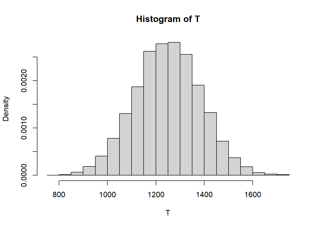

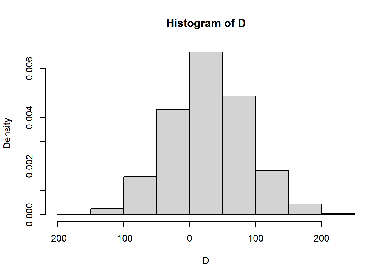
D = M - R

mean(D)

[1] 29.52545

sd(D)

[1] 59.12068

sum(D > 0) / N_rep

[1] 0.6928

hist(D,
     freq = FALSE)