Homework 5
Problem 1
(Continuing from a previous HW) The latest series of collectible Lego Minifigures contains 3 different Minifigure prizes (labeled 1, 2, 3). Each package contains a single unknown prize. Suppose we only buy 3 packages and we consider as our sample space outcome the results of just these 3 packages (prize in package 1, prize in package 2, prize in package 3). For example, 323 (or (3, 2, 3)) represents prize 3 in the first package, prize 2 in the second package, prize 3 in the third package. Let \(X\) be the number of distinct prizes obtained in these 3 packages. Let \(Y\) be the number of these 3 packages that contain prize 1. Suppose that each package is equally likely to contain any of the 3 prizes, regardless of the contents of other packages; let \(\text{P}\) denote the corresponding probability measure.
- Find the conditional distribution of \(Y\) given \(X=x\) for each possible value of \(x\) of \(X\).
- Compute and interpret \(\text{E}(Y|X=x)\) for each possible value of \(x\) of \(X\).
- Find the conditional distribution of \(X\) given \(Y=y\) for each possible value of \(y\) of \(Y\).
- Compute and interpret \(\text{E}(X|Y=y)\) for each possible value of \(y\) of \(Y\).
- Explain how you could use spinners to implement the “marginal then conditional” method to simulate an \((X, Y)\) pair.
- Suppose you have simulated many \((X, Y)\) pairs. Explain how you could use the simulation results to approximate:
- \(\text{P}(X = 1 | Y = 0)\)
- the conditional distribution of \(X\) given \(Y=0\)
- \(\text{E}(X = 1 | Y = 0)\)
Solution
Each row of the table below represents a different conditional distribution of \(Y\) given \(X=x\). For example, the row for \(x=1\) represents the conditional distribution of \(Y\) given \(X=1\): Given \(X=1\), \(Y\) is 0 with probability 2/3 and 3 with probability 1/3.
\(y\) 0 1 2 3 Total \(x\) 1 2/3 0 0 1/3 1 2 1/3 1/3 1/3 0 1 3 0 1 0 0 1 Take expected values according to each conditional distribution. In general, \(\text{E}(Y|X=x)\) depends on \(x\), but in this case \(\text{E}(Y|X=x) = 1\) for all values of \(x\).; regardless of how many distinct prizez people obtain in their, the average number of prize 1s obtains is 1.
\[\begin{align*} x & \quad \text{E}(Y|X=x)\\ 1 & \quad 0(2/3) + 3(1/3) = 1\\ 2 & \quad 0(1/3) + 1(1/3) + 2(1/3) = 1\\ 3 & \quad 1(1) = 1 \end{align*}\]
Each column of the table below represents a different conditional distribution of \(X\) given \(Y=y\). For example, the column for \(y=1\) represents the conditional distribution of \(X\) given \(Y=1\): Given \(Y=1\), \(X\) is 1 with probability 1/4 and 2 with probability 3/4.
\(y\) 0 1 2 3 \(x\) 1 1/4 0 0 1 2 3/4 1/2 1 0 3 0 1/2 0 0 Total 1 1 1 1 Take expected values according to each conditional distribution. For example, \(\text{E}(X|Y = 0) = 1.75\); among the people who never get prize 1 in their 3 boxes, the average number of distinct prizes they obtain is 1.75.
\[\begin{align*} y & \quad \text{E}(X|Y=y)\\ 0 & \quad 1(1/4) + 2(3/4) = 1.75\\ 1 & \quad 2(1/2) + 3(1/2) = 2.5\\ 2 & \quad 2(1) = 2\\ 3 & \quad 1(1) = 1 \end{align*}\]
Simulate a value of \(X\) from its marginal distribution: 1, 2, 3 with probability 3/27, 18/27, 6/27 (see previous HW for spinner). Given the value of \(x\), simulate \(Y\) from the appropriate conditional distribution of \(Y\) given \(X=x\):
- if \(x =1\), simulate \(Y\) from a spinner that returns values 0, 3 with probability 2/3, 1/3
- if \(x = 2\), simulate \(Y\) from a spinner that returns values 0, 1, 2 with probability 1/3, 1/3, 1/3
- if \(x =3\) then \(Y\) is 1 with probability 1.
- (You could also simulate \(Y\) first and then given \(Y=y\) simulate \(X\) from the appropriate conditional distribution of \(X\) given \(Y=y\).)
Simulate many \((X, Y)\) pairs using any appropriate method.
- Discard all pairs for which \(Y\) is not 0, count the number of remaining pairs in which \(X=1\) and divide by the number of non-discarded pairs (all with \(Y=0\)).
- Discard all pairs for which \(Y\) is not 0, and summarize the \(X\) values to find the conditional relative frequency of each possible \(X\) value as in the previous part (given \(Y=0\), the possible values of \(X\) are 1 and 2).
- Discard all pairs for which \(Y\) is not 0 and sum all the \(X\) values for the remaining pairs and divide by the number of non-discarded pairs to find the conditional average.
- (In all the above, be careful about the margin of error.)
Problem 2
Xavier and Yolanda are playing roulette. They both place bets on red on the same 3 spins of the roulette wheel before Xavier has to leave. (Remember, the probability that any bet on red on a single spin wins is 18/38.) After Xavier leaves, Yolanda places bets on red on 2 more spins of the wheel. Let \(X\) be the number of bets that Xavier wins and let \(Y\) be the number that Yolanda wins.
- Identify by name the marginal distribution of \(X\). Be sure to specify the values of any relevant parameters. Compute \(\text{E}(X)\).
- Identify by name the marginal distribution of \(Y\). Be sure to specify the values of any relevant parameters. Compute \(\text{E}(Y)\).
- The joint distribution of \(X\) and \(Y\) is represented in the table below. Explain why \(p_{X, Y}(1, 4) = 0\) and \(p_{X, Y}(2, 1) = 0\).
- Compute \(p_{X, Y}(2, 3)\). (Yes, the table tells you it’s 0.1766, but you have to show how this number can be computed based on the assumptions of the problem.)
- Are \(X\) and \(Y\) independent? Justify your answer with an appropriate calculation.
- Compute and interpret \(\text{P}(X + Y) = 4\).
- Make a table representing the marginal distribution of \(X+Y\).
- Use the table from the previous part to compute \(\text{E}(X+Y)\), and verify that it is equal to \(\text{E}(X)+\text{E}(Y)\).
- Without doing any computation, determine if \(\text{Var}(X+Y)\) will be greater than, less than, or equal to \(\text{Var}(X) + \text{Var}(Y)\). Explain your reasoning.
| \(x\), \(y\) | 0 | 1 | 2 | 3 | 4 | 5 |
|---|---|---|---|---|---|---|
| 0 | 0.0404 | 0.0727 | 0.0327 | 0 | 0 | 0 |
| 1 | 0 | 0.109 | 0.1963 | 0.0883 | 0 | 0 |
| 2 | 0 | 0 | 0.0981 | 0.1766 | 0.0795 | 0 |
| 3 | 0 | 0 | 0 | 0.0294 | 0.053 | 0.0238 |
Solution
\(X\) has a Binomial distribution with parameters \(n=3\) and \(p = 18/38\), so \(\text{E}(X) = np = 3(18/38) = 1.42\).
\(Y\) has a Binomial distribution with parameters \(n=5\) and \(p = 18/38\), so \(\text{E}(X) = np = 5(18/38) = 2.37\).
In the first 3 bets Yolanda wins the same number of games as Xavier, and Yolanda only plays two more games. So \(Y\) can’t be more than \(X+2\), and \(Y\) can’t be less than \(X\).
To have \(X = 2\) and \(Y=3\) we need to have exactly two wins in the first 3 bets (where both play) exactly 1 win in the last 2 bets (Yolanda only). The number of wins in the first 3 bests is Binomial(3, 18/38), the number of wins in the last two bets is Binomial(2, 18/38) and the first 3 bets are independent of the last two bets. So the probability is
dbinom(2, 3, 18 / 38) * dbinom(1, 2, 18 / 38)= 0.177 or \[ p_{X, Y}(2, 3) = \text{P}(X = 2, Y = 3) = \left(\binom{3}{1}(18/38)^2(20/38)^1\right)\left(\binom{2}{1}(18/38)^1(20/38)^1\right) = 0.177 \]No. \(X\) and \(Y\) are not independent. For example \(\text{P}(X = 0) = 0.15\) but \(\text{P}(X=0|Y = 0) = 1\).
Sum over the \((X, Y)\) pairs for which \(X + Y = 4\): (0, 4), (1, 3), (2, 2), (3, 1), (4, 0). So 0 + 0.0883 + 0.0981 + 0 = 0.1864. Suppose they do this every time they visit the casino. Over many visits to the casino, together they win a total of 4 bets in 18.6% of visits
The possible values are \(0, 1, \ldots, 8\). Fill in the probabilities like in the previous part. (Alternative \(X + Y\) has the same distribution as \(2X + Z\) where \(X\) and \(Z\) are independent and \(Z\) (number of wins in last two bets) has a Binomial(2, 18/38) distribution).
Value Probability 0 0.0404 1 0.0727 2 0.1417 3 0.1963 4 0.1864 5 0.1766 6 0.1089 7 0.0530 8 0.0238 From the table \(\text{E}(X+Y) = 0(0.404) + 1(0.0727 + \cdots + 8(0.0238) = 3.79\), and \(\text{E}(X)+\text{E}(Y) = 3(18/38) + 5(18/38) = 3.79\). (These are exactly equal; any differences are just rounding errors)
There is a positive association so \(\text{Var}(X+Y)\) will be greater than \(\text{Var}(X) + \text{Var}(Y)\).
Problem 3
Percent returns for assets \(X\), \(Y\), and \(Z\) follow a joint distribution with
- Mean 10 and standard deviation 15 for asset X,
- Mean 5 and standard deviation 3 for asset Y,
- Correlation of −0.6 between asset X and asset Y
- Asset Z yields a constant return of 1 percent.
An investment portfolio has 60% of its funds in asset X, 30% in asset Y, and 10% in asset Z.
- Let \(R\) be the portfolio return. Express \(R\) in terms of \(X, Y, Z\).
- Compute \(\text{E}(R)\).
- Compute \(\text{Cov}(X, Y)\).
- Compute \(\text{Cov}(X, Z)\).
- Compute \(\text{SD}(R)\).
Solution
- \(R = 0.6X + 0.3Y + 0.1Z\)
- Linearity of expected value \[ \text{E}(R)=\text{E}(0.6X + 0.3Y + 0.1Z) = 0.6\text{E}(X) + 0.3\text{E}(Y) + 0.1\text{E}(Z) = 0.6(10) + 0.3(5) + 0.1(1) = 7.6 \]
- \(\text{Cov}(X, Y) = \text{Corr}(X, Y)\text{SD}(X)\text{SD}(Y) = (-0.6)(15)(3) = -27\)
- \(Z\) is constant so \(\text{Cov}(X, Z)=0\)
- Use properties of variance and covariance \[\begin{align*} & \text{Var}(0.6X + 0.3Y + 0.1Z) & & \\ & = \text{Var}(0.6X + 0.3Y) & & \text{$Z$ is constant, no affect variability}\\ & = \text{Var}(0.6X) + \text{Var}(0.3Y) + 2\text{Cov}(0.6X, 0.3Y) & & \text{variance of sum}\\ & = 0.6^2\text{Var}(X) + 0.3^2\text{Var}(Y) + 2(0.6)(0.3)\text{Cov}(X, Y) && \text{rules for variance}\\ & = 0.6^2\text{SD}(X)^2 + 0.3^2\text{SD}(Y)^2 + 2(0.6)(0.3)\text{Corr}(X, Y)\text{SD}(X)\text{SD}(Y) && \text{correlation}\\ & = 0.6^2(15^2) + 0.3^2(3)^2 + 2(0.6)(0.3)(-0.6)(15)(3) & & \\ & = 72.09 \end{align*}\] So \(\text{SD}(R) = \sqrt{\text{Var}(R)} = \sqrt{72} = 8.49\).
Problem 4
Devi and Paxton are meeting. Arrival times are measured in minutes after noon, with negative times representing arrivals before noon. Devi’s arrival time follows a Normal distribution with mean 20 and SD 15 minutes, and Paxton’s arrival time follows a Normal distribution with mean 25 and SD 10 minutes, independently of each other.
For each of the following, find the appropriate standardized value and make a ballpark estimate of the probability. Then use software to compute the probability.
- Compute the probability that Devi arrives before noon.
- Compute the probability that Devi arrives first.
- Compute the probability that the first person to arrive has to wait more than 15 minutes for the second person to arrive.
- Coding required. Code and run a simulation and use the results to approximate the probability from the previous part (just part c). You should first simulate (Devi, Paxton) arrival time pairs, and go from there.
Solution
- If \(V\) is Devi’s arrival time, \(V\sim N(20, 15)\). We want \(\text{P}(V < 0)\). The standardized value for 0 is \((0 - 20)/15=-1.333\); that is, 0 is 1.333 SDs below the mean. From the empirical rule, 87% of values are within 1.5 SDs of the mean, so our estimated probability is more than 6.5%. For software, see below; \(\text{P}(V < 0)=0.09\).
- If \(X\) is Paxton’s arrival time, we want \(\text{P}(X > V) = \text{P}(X - V >0)\). Since \(X\) and \(V\) are independent each with a Normal distribution, then \(X - V\) has a Normal distribution. The mean is \(20-15 = 5\), and since \(X\) and \(V\) are independent \[ \text{Var}(X - V) = \text{Var}(X) + \text{Var}(V) - 2\text{Cov}(X, V) = 10^2 + 15^2 - 0 = 325 \] So \(\text{SD}(X - V) = \sqrt{325} = 18.0\). We want \(\text{P}(X - V > 0)\). The standardized value for 0 is \((0 - 5)/18=-0.277\); that is, 0 is 0.277 SDs below the mean. The probability will be more than 50%. For software, see below; \(\text{P}(X - V > 0)=0.61\).
- We want \(\text{P}(|X - V| >15) = \text{P}(X - V > 15) + \text{P}(X - V < -15)\). The standardized value for 15 is \((15 - 5) / 18 = 0.556\). The standardized value for -15 is \((-15 - 5) / 18 = -1.11\). The probability that a value is more than 1 SD below the mean is about 0.16; the probability that a value is more than 0.5 SDs above the mean is about 0.31. So the probability that we want is less than 0.47. It’s \(\text{P}(|X - V| > 15) = 0.42\).
pnorm((0 - 20) / 15)[1] 0.09121122pnorm(0, 20, 15)[1] 0.091211221 - pnorm((0 - 5) / 18)[1] 0.60940851 - pnorm(0, 5, 18)[1] 0.60940851 - pnorm((15 - 5) / 18) + pnorm((-15 - 5) / 18)[1] 0.42251761 - pnorm(15, 5, 18) + pnorm(-15, 5, 18)[1] 0.4225176N_rep = 10000
V = rnorm(N_rep, 20, 15)
X = rnorm(N_rep, 25, 10)
sum(abs(V - X) > 15) / N_rep[1] 0.4257cor(V, X)[1] -0.0351468mean(V)[1] 19.97441sd(V)[1] 14.94365mean(X)[1] 24.91276sd(X)[1] 9.970663plot(V, X, col = ifelse(abs(V - X) > 15, "orange", "gray"))
abline(a = 15, b = 1, col = "orange")
abline(a = -15, b = 1, col = "orange")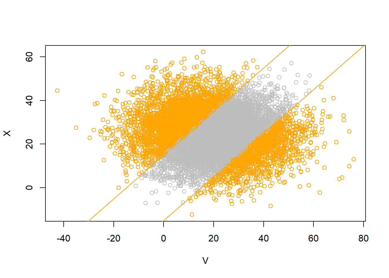
ggplot(data.frame(V, X), aes(x = V, y = X)) +
  stat_density_2d(aes(fill = ..level..), geom = "polygon", colour="white") +
  geom_abline(slope = 1, intercept = c(-15, 15), col = "orange", size = 2)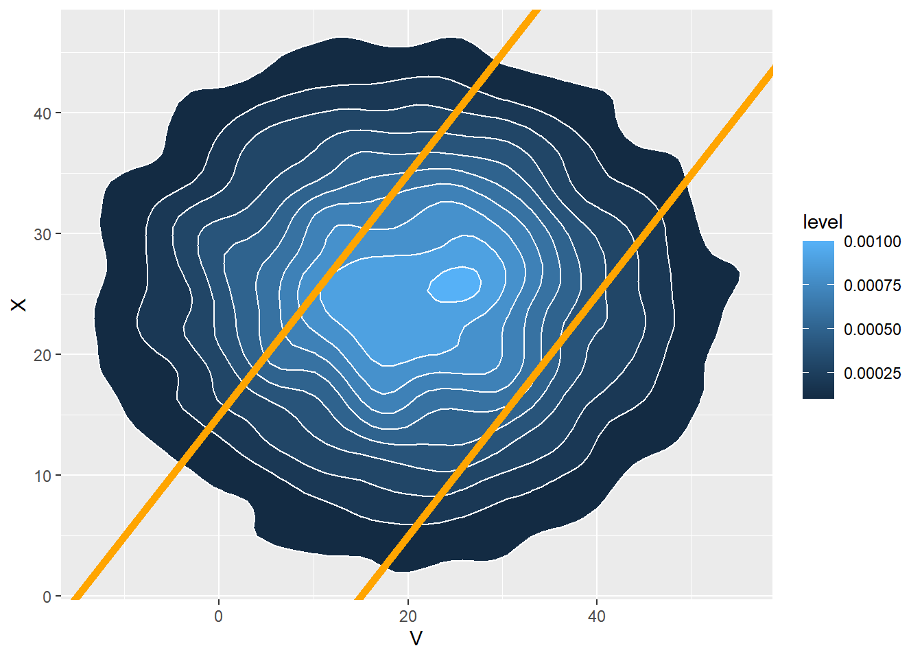
Problem 5 part 1
(Continued.) Devi and Paxton are meeting. Arrival times are measured in minutes after noon, with negative times representing arrivals before noon. Devi’s arrival time follows a Normal distribution with mean 20 and SD 15 minutes, and Paxton’s arrival time follows a Normal distribution with mean 25 and SD 10 minutes.
For each of the following, find the appropriate standardized value and make a ballpark estimate of the probability. Then use software to compute the probability.
Assume the pairs of arrival times follow a Bivariate Normal distribution with correlation 0.8
- Compute the probability that Devi arrives first given that Paxton arrives at 12:10.
- Compute the probability that the first person to arrive has to wait more than 15 minutes for the second person to arrive.
- Coding required. Code and run a simulation and use the results to approximate the probability from the previous part (just part b). You should first simulate (Devi, Paxton) arrival time pairs, and go from there.
Solution
Let \(V\) be Devi’s arrival time and let \(X\) be Paxton’s arrival time.
- We want \(\text{P}(V < X | X = 10) = \text{P}(V < 10 | X = 10)\). Paxton’s time is 1.5 SDs below the mean, \(\frac{10 - 25}{10} = -1.5\). Devi’s conditional mean arrival time is 1.2 SDs below the mean, \(0.8(-1.5) = -1.2\), so Devi’s conditional mean arrival time is \(\text{E}(V | X = 10) = 20 -1.2(15) =2\). Devi’s conditional SD is \(\text{SD}(V|X = 10) = 15\sqrt{1-0.8^2} = 9\). So \((V | (X = 10))\sim N(2, 9)\). \(\text{P}(V < 10 | X = 10) = \text{P}(Z < \frac{10-2}{9}) = \text{P}(Z < 0.889)\); ballpark estimate a little less than 84%. Software (below) gives 0.81.
- We want \(\text{P}(|X - V| >15) = \text{P}(X - V > 15) + \text{P}(X - V < -15)\). Since \(X\) and \(V\) have a Bivariate Normal distribution, then \(X - V\) has a Normal distribution. The mean is \(20-15 = 5\), and \[ \text{Var}(X - V) = \text{Var}(X) + \text{Var}(V) - 2\text{Cov}(X, V) = 10^2 + 15^2 - 2(0.8)(10)(15) = 85 \] So \(\text{SD}(X - V) = \sqrt{85} = 9.2\). The standardized value for 15 is \((15 - 5) / 9.2 = 1.08\). The standardized value for -15 is \((-15 - 5) / 9.2 = -2.17\). The probability that a value is more than 2 SDs below the mean is about 0.025; the probability that a value is more than 1 SD above the mean is about 0.16. So the probability that we want is less than 0.185. It’s \(\text{P}(|X - V| > 15) = 0.15\).
pnorm((10 - 2) / 9)[1] 0.8129686pnorm(10, 2, 9)[1] 0.81296861 - pnorm((15 - 5) / 9.2) + pnorm((-15 - 5) / 9.2)[1] 0.15338381 - pnorm(15, 5, 9.2) + pnorm(-15, 5, 9.2)[1] 0.1533838N_rep = 10000
V = rnorm(N_rep, 20, 15)
X = rnorm(N_rep, 25 + 10 * 0.8 * (V - 20) / 15, 10 * sqrt(1 - 0.8 ^ 2))
sum(abs(V - X) > 15) / N_rep[1] 0.1564cor(V, X)[1] 0.8030264mean(V)[1] 19.88082sd(V)[1] 15.03541mean(X)[1] 24.86761sd(X)[1] 10.06431plot(V, X, col = ifelse(abs(V - X) > 15, "orange", "gray"))
abline(a = 15, b = 1, col = "orange")
abline(a = -15, b = 1, col = "orange")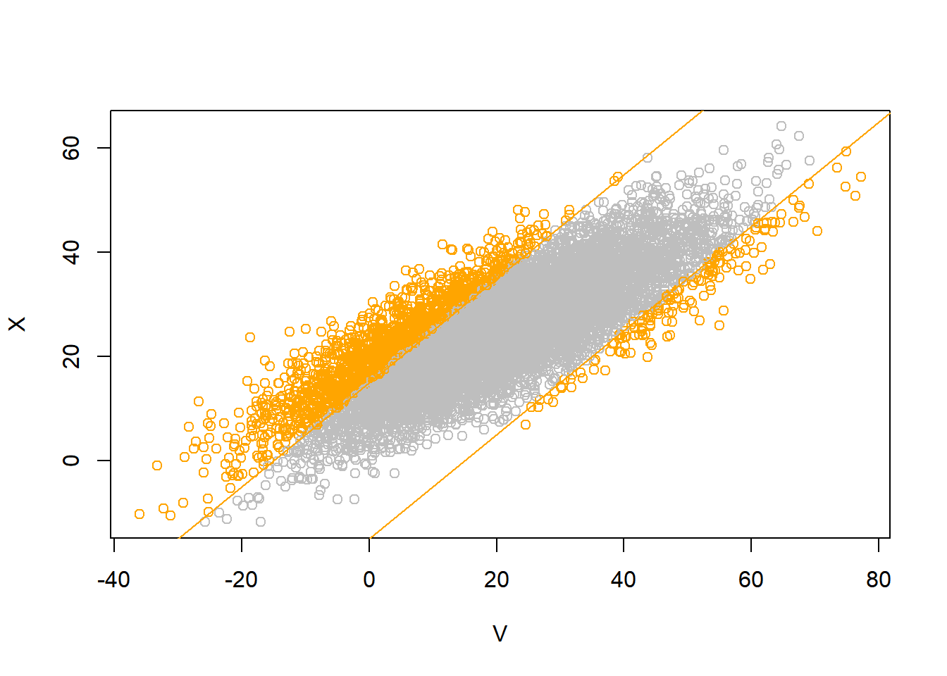
ggplot(data.frame(V, X), aes(x = V, y = X)) +
  stat_density_2d(aes(fill = ..level..), geom = "polygon", colour="white") +
  geom_abline(slope = 1, intercept = c(-15, 15), col = "orange", size = 2)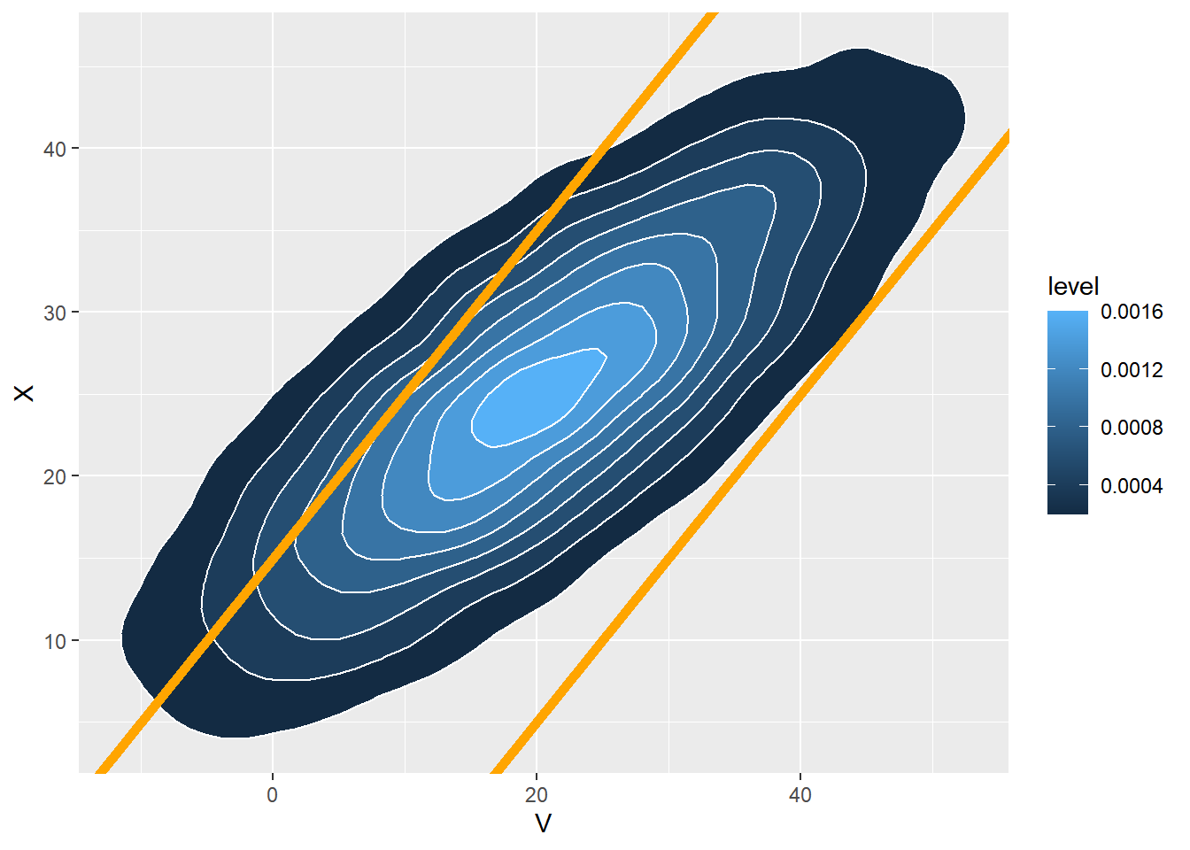
Problem 5 part 2
(Continued.) Devi and Paxton are meeting. Arrival times are measured in minutes after noon, with negative times representing arrivals before noon. Devi’s arrival time follows a Normal distribution with mean 20 and SD 15 minutes, and Paxton’s arrival time follows a Normal distribution with mean 25 and SD 10 minutes.
For each of the following, find the appropriate standardized value and make a ballpark estimate of the probability. Then use software to compute the probability.
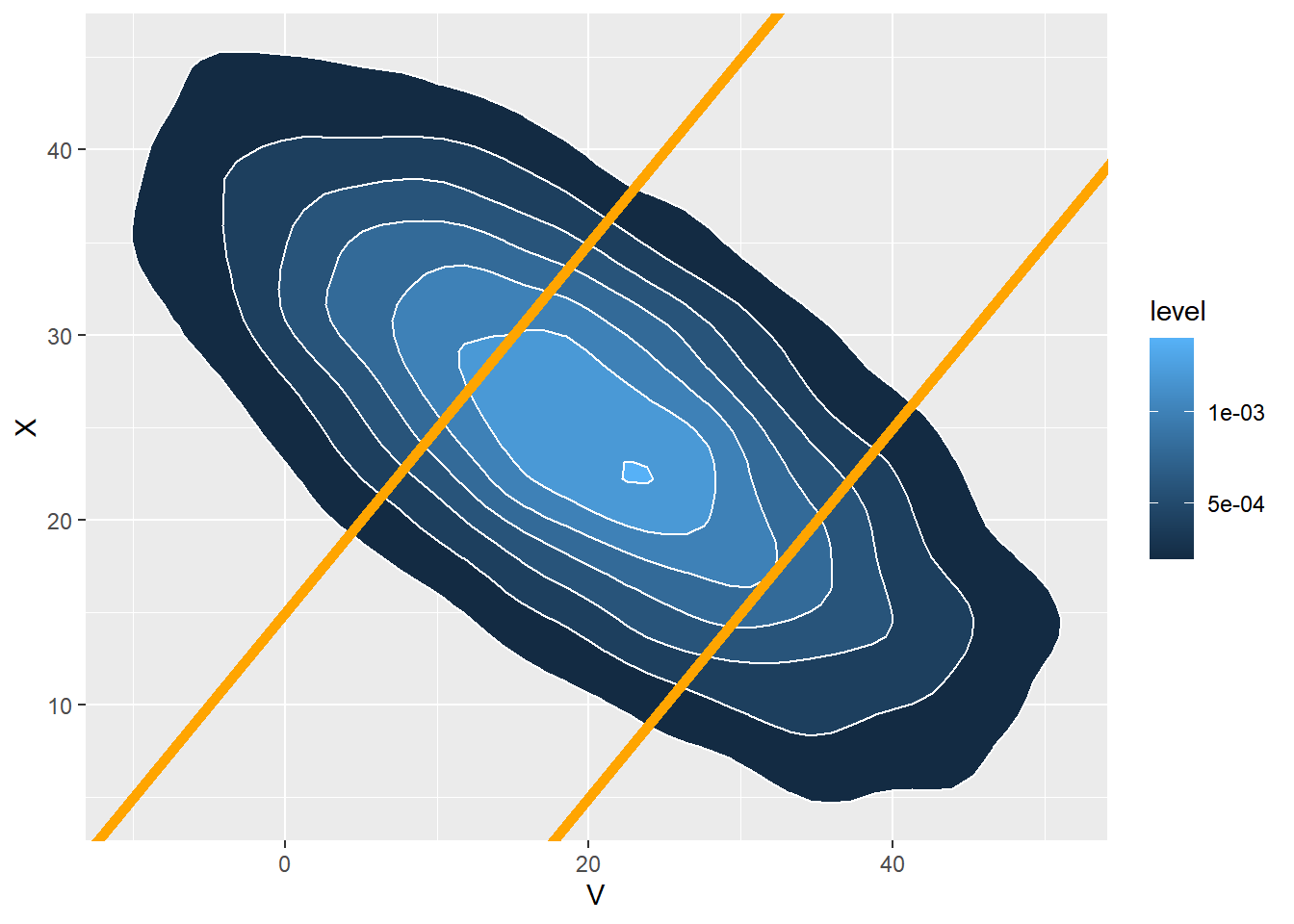
Assume the pairs of arrival times follow a Bivariate Normal distribution with correlation -0.7
- Compute the probability that Devi arrives first given that Paxton arrives at 12:10.
- Compute the probability that the first person to arrive has to wait more than 15 minutes for the second person to arrive.
- Coding required. Code and run a simulation and use the results to approximate the probability from the previous part (just part b). You should first simulate (Devi, Paxton) arrival time pairs, and go from there.
Solution
- We want \(\text{P}(V < X | X = 10) = \text{P}(V < 10 | X = 10)\). Paxton’s time is 1.5 SDs below the mean, \(\frac{10 - 25}{10} = -1.5\). Devi’s conditional mean arrival time is 1.05 SDs above the mean, \((-0.7)(-1.5) = 1.05\), so Devi’s conditional mean arrival time is \(\text{E}(V | X = 10) = 20 +1.05(15) =35.75\). Devi’s conditional SD is \(\text{SD}(V|X = 10) = 15\sqrt{1-0.7^2} = 10.7\). So \((V | (X = 10))\sim N(35.75, 10.7)\). \(\text{P}(V < 10 | X = 10) = \text{P}(Z < \frac{10-35.75}{10.7}) = \text{P}(Z < -2.4)\); ballpark estimate is about 0.005. Software (below) gives 0.008.
- We want \(\text{P}(|X - V| >15) = \text{P}(X - V > 15) + \text{P}(X - V < -15)\). Since \(X\) and \(V\) have a Bivariate Normal distribution, then \(X - V\) has a Normal distribution. The mean is \(20-15 = 5\), and \[ \text{Var}(X - V) = \text{Var}(X) + \text{Var}(V) - 2\text{Cov}(X, V) = 10^2 + 15^2 - 2(-0.7)(10)(15) = 535 \] So \(\text{SD}(X - V) = \sqrt{535} = 23.1\). The standardized value for 15 is \((15 - 5) / 23.1 = 0.43\). The standardized value for -15 is \((-15 - 5) / 23.1 = -0.86\). The probability that a value is more than 1 SD below the mean is about 0.16; the probability that a value is more than 0.5 SD above the mean is about 0.31. So the probability that we want is about 0.47. It’s \(\text{P}(|X - V| > 15) = 0.53\).
pnorm((10 - 35.75) / 10.7)[1] 0.008052175pnorm(10, 35.75, 10.7)[1] 0.0080521751 - pnorm((15 - 5) / 23.1) + pnorm((-15 - 5) / 23.1)[1] 0.52584321 - pnorm(15, 5, 23.1) + pnorm(-15, 5, 23.1)[1] 0.5258432N_rep = 10000
V = rnorm(N_rep, 20, 15)
X = rnorm(N_rep, 25 + 10 * (-0.7) * (V - 20) / 15, 10 * sqrt(1 - 0.7 ^ 2))
sum(abs(V - X) > 15) / N_rep[1] 0.5296cor(V, X)[1] -0.701365mean(V)[1] 19.8809sd(V)[1] 15.05062mean(X)[1] 25.1412sd(X)[1] 10.00519plot(V, X, col = ifelse(abs(V - X) > 15, "orange", "gray"))
abline(a = 15, b = 1, col = "orange")
abline(a = -15, b = 1, col = "orange")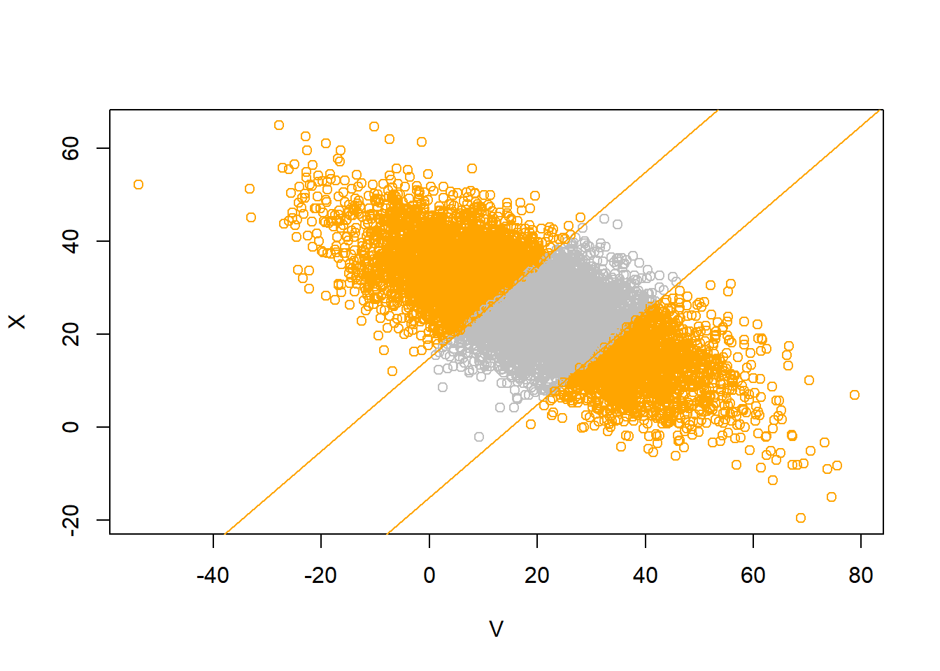
ggplot(data.frame(V, X), aes(x = V, y = X)) +
  stat_density_2d(aes(fill = ..level..), geom = "polygon", colour="white") +
  geom_abline(slope = 1, intercept = c(-15, 15), col = "orange", size = 2)