2 Working with Probabilities

Due to the wide variety of types of random phenomena, an outcome can be virtually anything. In particular, an outcome does not have to be a number.
The sample space is the set of all possible outcomes of the random phenomenon..
An event is something that could happen. That is, an event is a collection of outcomes that satisfy some criteria. If the sample space outcomes are represented by rows in a spreadsheet, then an event is a subset of rows that satisfies some criteria
Events are typically denoted with capital letters near the start of the alphabet, with or without subscripts (e.g. $A$, $B$, $C$, $A_1$, $A_2$). Events can be composed from others using basic set operations like unions ($A\cup B$), intersections ($A \cap B$), and complements ($A^c$).
- Read $A^c$ as “not $A$”.
- Read $A\cap B$ as “$A$ and $B$”
- Read $A \cup B$ as “$A$ or $B$”. Note that unions ($\cup$, “or”) are always inclusive. $A\cup B$ occurs if $A$ occurs but $B$ does not, $B$ occurs but $A$ does not, or both $A$ and $B$ occur.
A collection of events $A_1, A_2, \ldots$ are disjoint (a.k.a. mutually exclusive) if $A_i \cap A_j = \emptyset$ for all $i \neq j$. That is, multiple events are disjoint if none of the events have any outcomes in common.
A probability measure, typically denoted $\text{P}$, assigns probabilities to events to quantify their relative likelihoods according to the assumptions of the model of the random phenomenon.
The probability of event $A$, computed according to probability measure $\text{P}(A)$, is denoted $\text{P}(A)$.
A valid probability measure $\text{P}$ must satisfy the following three logical consistency “axioms”.
- For any event $A$, $0 \le \text{P}(A) \le 1$.
- If $\Omega$ represents the sample space then $\text{P}(\Omega) = 1$.
- (Countable additivity.) If $A_1, A_2, A_3, \ldots$ are disjoint then \[ \text{P}(A_1 \cup A_2 \cup A_2 \cup \cdots) = \text{P}(A_1) + \text{P}(A_2) +\text{P}(A_3) + \cdots \]
Additional properties of a probability measure follow from the axioms
- Complement rule. For any event $A$, $\text{P}(A^c) = 1 - \text{P}(A)$.
- Subset rule. If $A \subseteq B$ then $\text{P}(A) \le \text{P}(B)$.
- Addition rule for two events. If $A$ and $B$ are any two events \[ \text{P}(A\cup B) = \text{P}(A) + \text{P}(B) - \text{P}(A \cap B) \]
- Law of total probability. If $C_1, C_2, C_3\ldots$ are disjoint events with $C_1\cup C_2 \cup C_3\cup \cdots =\Omega$, then \[ \text{P}(A) = \text{P}(A \cap C_1) + \text{P}(A \cap C_2) + \text{P}(A \cap C_3) + \cdots \]
The axioms of a probability measure are minimal logical consistent requirements that ensure that probabilities of different events fit together in a valid, coherent way.
A single probability measure corresponds to a particular set of assumptions about the random phenomenon.

Example 2.1

The probability that a randomly selected U.S. household has a pet dog is 0.47. The probability that a randomly selected U.S. household has a pet cat is 0.25. (These values are based on the 2018 General Social Survey (GSS).)

Represent the information provided using proper symbols.
Donny Don’t says: “the probability that a randomly selected U.S. household has a pet dog OR a pet cat is $0.47 + 0.25=0.72$.” Do you agree? What must be true for Donny to be correct? Explain. (Hint: for the remaining parts it helps to consider two-way tables.)
What is the largest possible value of the probability that a randomly selected U.S. household has a pet dog AND a pet cat? Describe the (unrealistic) situation in which this extreme case would occur.
What is the smallest possible value of the probability that a randomly selected U.S. household has a pet dog AND a pet cat? Describe the (unrealistic) situation in which this extreme case would occur.
Donny Don’t says: “I remember hearing once that in probability OR means add and AND means multiply. So the probability that a randomly selected U.S. household has a pet dog AND a pet cat is $0.47 \times 0.25=0.1175$.” Do you agree? Explain.
According to the GSS, the probability that a randomly selected U.S. household has a pet dog AND a pet cat is $0.15$. Compute the probability that a randomly selected U.S. household has a pet dog OR a pet cat.
Compute and interpret $\text{P}(C \cap D^c)$.

2.1 Equally Likely Outcomes and Uniform Probability Measures

For a sample space $\Omega$ with finitely many possible outcomes, assuming equally likely outcomes corresponds to a probabiliy measure $\text{P}$ which satisfies

\[ \text{P}(A) = \frac{|A|}{|\Omega|} = \frac{\text{number of outcomes in $A$}}{\text{number of outcomes in $\Omega$}} \qquad{\text{when outcomes are equally likely}} \]

Example 2.2

Roll a fair four-sided die twice, and record the result of each roll in sequence.

How many possible outcomes are there? Are they equally likely?
Compute $\text{P}(A)$, where $A$ is the event that the sum of the two dice is 4.
Compute $\text{P}(B)$, where $B$ is the event that the sum of the two dice is at most 3.
Compute $\text{P}(C)$, where $C$ the event that the larger of the two rolls (or the common roll if a tie) is 3.
Compute and interpret $\text{P}(A\cap C)$.

Table 2.1: Table representing the sample space of two rolls of a four-sided die. The outcomes in orange comprise the event A, the sum is equal to 4.
First roll	Second roll	Sum is 4?
1	1	no
1	2	no
1	3	yes
1	4	no
2	1	no
2	2	yes
2	3	no
2	4	no
3	1	yes
3	2	no
3	3	no
3	4	no
4	1	no
4	2	no
4	3	no
4	4	no

The continuous analog of equally likely outcomes is a uniform probability measure. When the sample space is uncountable, size is measured continuously (length, area, volume) rather that discretely (counting).

\[ \text{P}(A) = \frac{|A|}{|\Omega|} = \frac{\text{size of } A}{\text{size of } \Omega} \qquad \text{if $\text{P}$ is a uniform probability measure} \]

Example 2.3

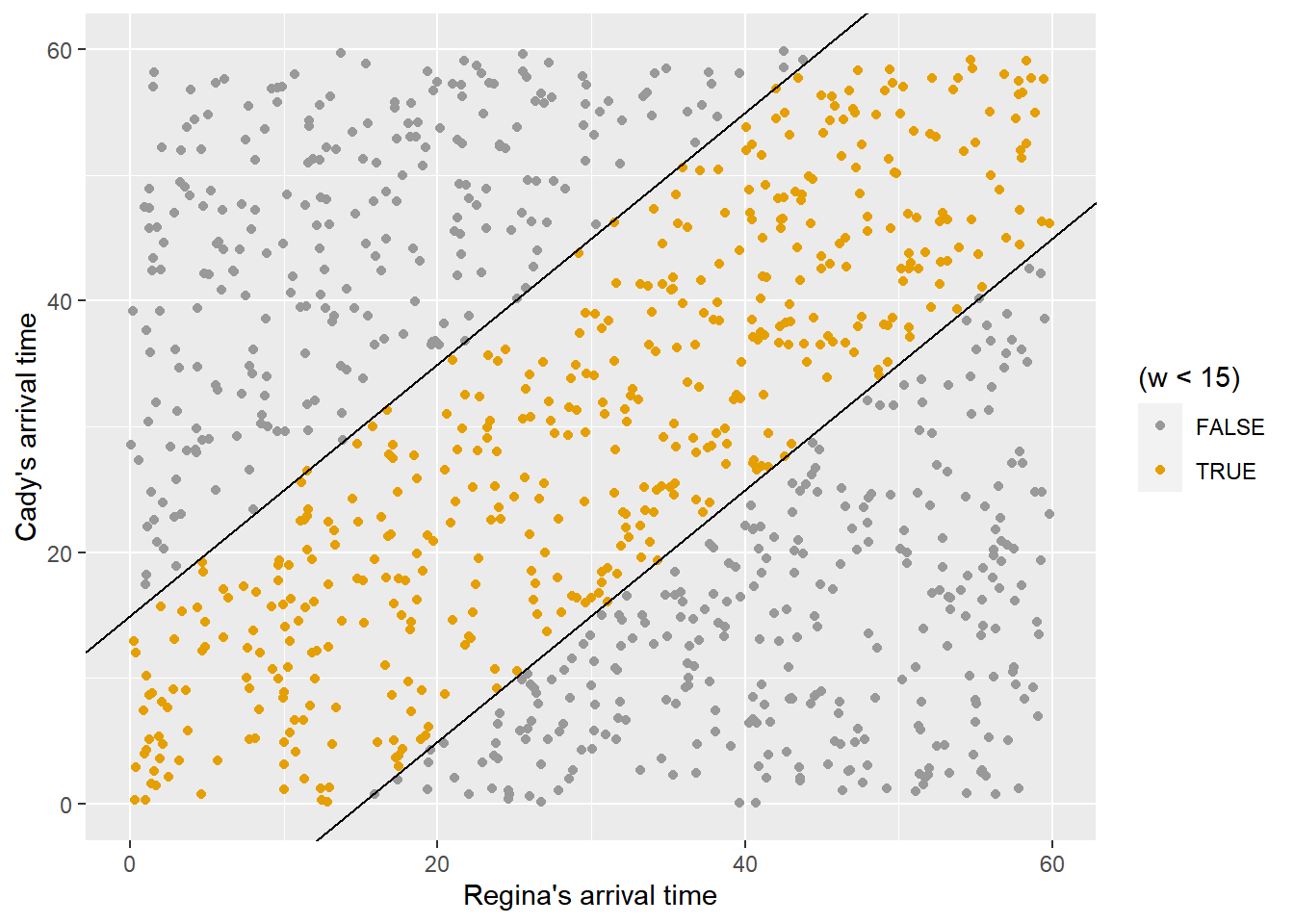
Regina and Cady are meeting for lunch. Suppose they each arrive uniformly at random at a time between noon and 1:00, independently of each other. Record their arrival times as minutes after noon, so noon corresponds to 0 and 1:00 to 60.

Draw a picture representing the sample space.
Compute the probability that the first person to arrive has to wait at most 15 minutes for the other person to arrive. In other words, compute the probability that they arrive within 15 minutes of each other.
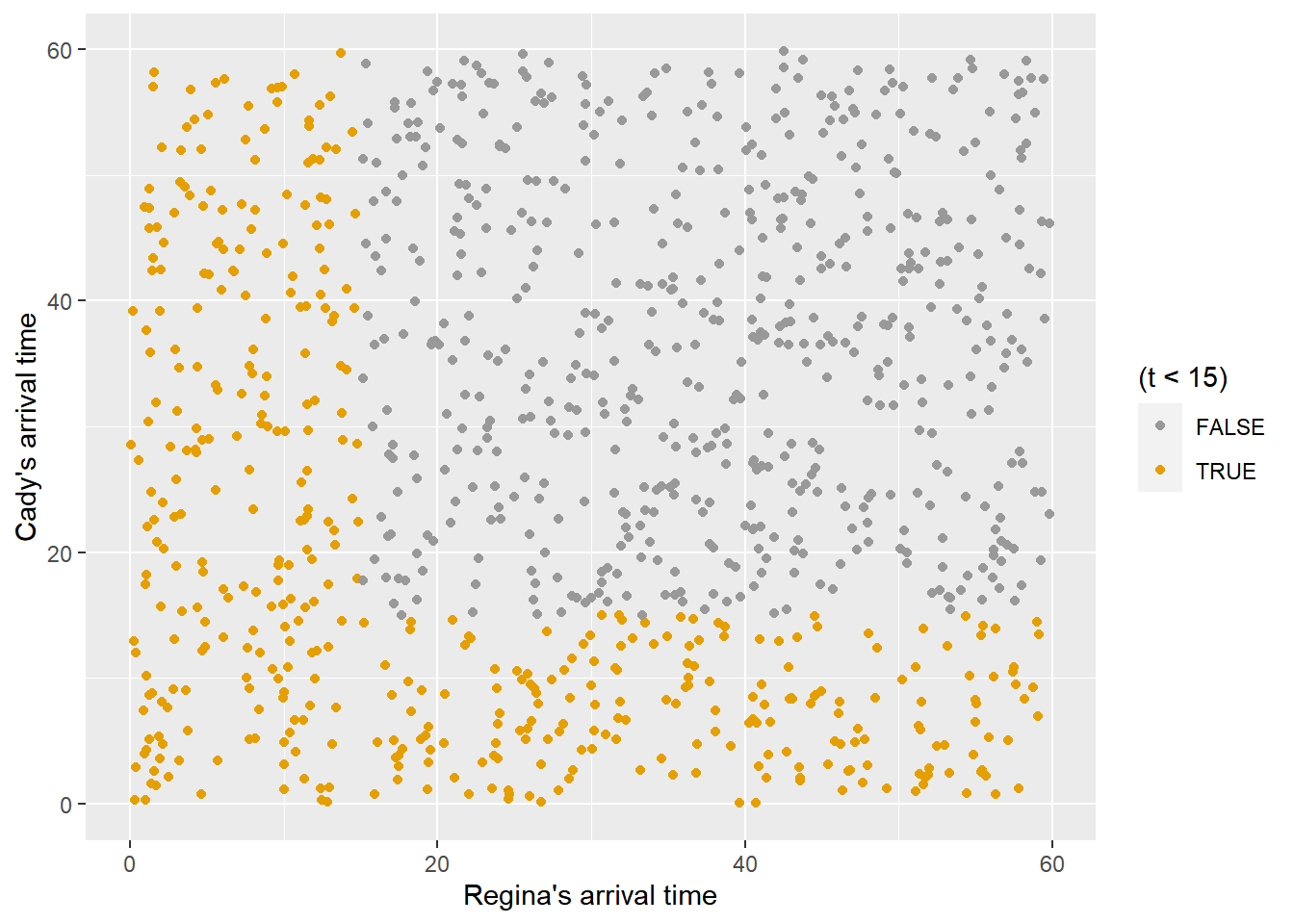
Compute the probability that the first person to arrive arrives before 12:15.

N_rep = 1000

# Simulate values uniformly between 0 and 60, independently
x = runif(N_rep, 0, 60)
y = runif(N_rep, 0, 60)

# waiting time
w = abs(x - y)

# first time
t = pmin(x, y)

# put the variables together in a data frame
meeting_sim = data.frame(x, y, w, t)

# first few rows (with kable formatting)
head(meeting_sim) |>
  kbl(digits = 3) |>
  kable_styling()

x	y	w	t
1.063	37.664	36.601	1.063
17.729	50.006	32.276	17.729
21.610	56.212	34.602	21.610
27.191	5.129	22.062	5.129
36.913	4.759	32.155	4.759
19.605	36.501	16.896	19.605

# Approximate probability that waiting time is less than 15
sum(w < 15) / N_rep

[1] 0.451

# Approximate probability that first arrival time is less than 15
sum(t < 15) / N_rep

[1] 0.442

# "Base R" plots
plot(x, y,
     col = ifelse(w < 15, "orange", "black"),
     xlab = "Regina's arrival time",
     ylab = "Cady's arrival time")
abline(a = 15, b = 1)
abline(a = -15, b = 1)

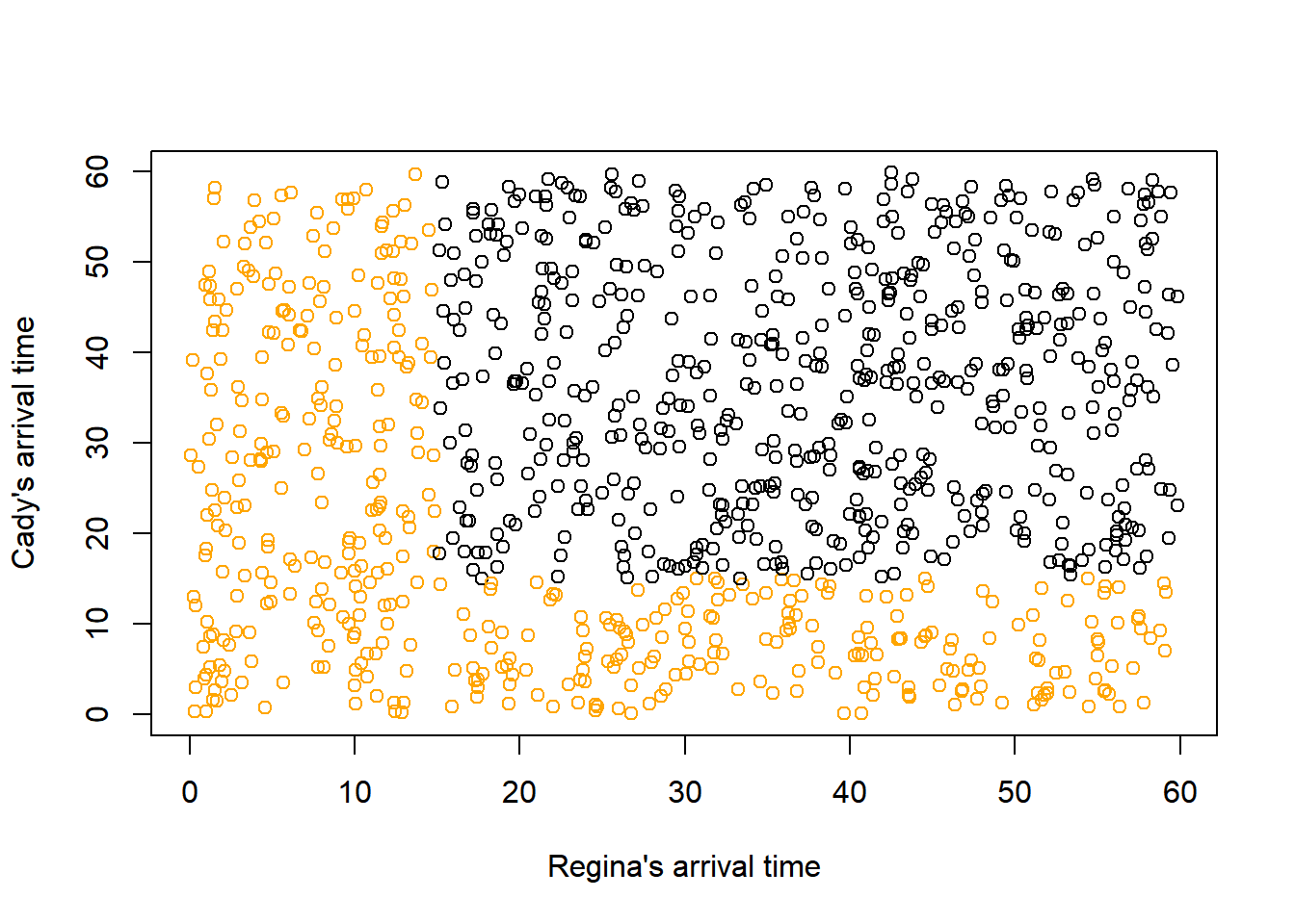
plot(x, y,
     col = ifelse(t < 15, "orange", "black"),
     xlab = "Regina's arrival time",
     ylab = "Cady's arrival time")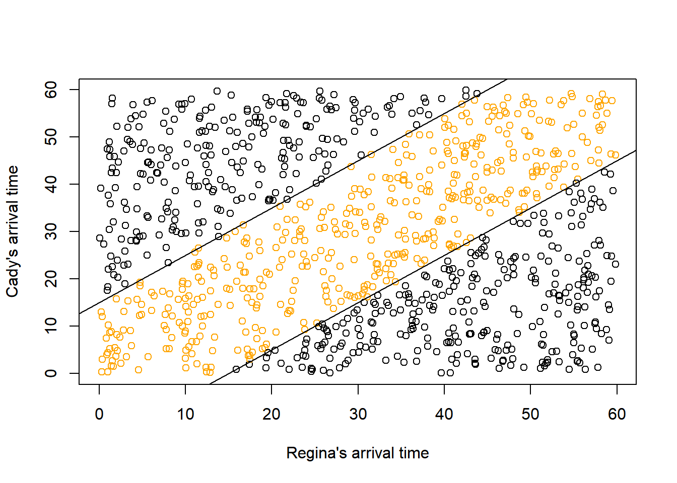

Simulated event that waiting time is less than 15

Simulated event that first arrival time is less than 15

library(ggplot2)

# ggplots
ggplot(meeting_sim,
       aes(x = x, y = y, col = (w < 15))) +
  geom_point() +
  geom_abline(slope = c(1,1), intercept = c(15, -15)) +
  labs(x = "Regina's arrival time",
       y = "Cady's arrival time")

ggplot(meeting_sim,
       aes(x = x, y = y, col = (t < 15))) +
  geom_point() +
  labs(x = "Regina's arrival time",
       y = "Cady's arrival time")