9  Continuous Random Variables: Probability Density Functions

• Simulated values of a continuous random variable are usually plotted in a histogram which groups the observed values into “bins” and plots densities or frequencies for each bin. (R: hist).
• In a histogram areas of bars represent relative frequencies; the axis which represents the height of the bars is called “density” (R: hist with freq = FALSE).
• The distribution of a continuous random variable can be described by a probability density function (pdf), for which areas under the density curve determine probabilities.

9.1 Uniform Distributions

Example 9.1

In the meeting problem assume that Regina’s arrival time $X$ (minutes after noon) follows a Uniform(0, 60) distribution. Figure 9.1 displays a histogram of 10000 simulated values of $X$.

N_rep = 10000

x = runif(N_rep, 0, 60)

data.frame(1:N_rep, x) |>
  head() |>
  kbl(col.names = c("Repetition", "X")) |>
  kable_styling(fixed_thead = TRUE)

Repetition	X
1	1.062914
2	17.729239
3	21.610468
4	27.190663
5	36.913450
6	19.604730

hist(x,
     freq = FALSE,
     main = "")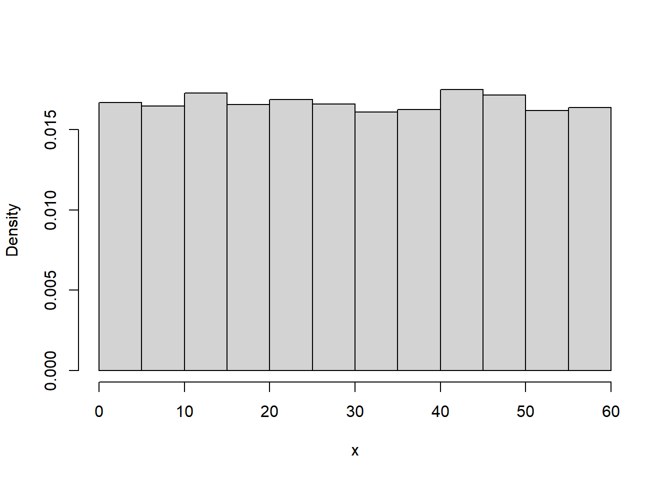

Figure 9.1: Simulated values from a Uniform(0, 60) distribution

1. Sketch a plot of the pdf of $X$.
   
   
   
   
   
2. Use the pdf to find the probability that Regina arrives before 12:15.
   
   
   
   
   
3. Use the pdf to find the probability that Regina arrives after 12:45.
   
   
   
   
   
4. Use the pdf to find the probability that Regina arrives between 12:15:00 and 12:16:00.
   
   
   
   
   
5. Use the pdf to find the probability that Regina arrives between 12:15:00 and 12:15:01.
   
   
   
   
   
6. Compute $\text{P}(X=15)$, the probability that Regina arrives at the exact time 12:15:00 (with infinite precision).
   
   
   
   
   

• The probability that a continuous random variable $X$ equals any particular value is 0. That is, if $X$ is continuous then $\text{P}(X=x)=0$ for all $x$.
• Even though any specific value of a continuous random variable has probability 0, intervals still can have positive probability.
• In practical applications involving continuous random variables, “equal to” really means “close to”, and “close to” probabilities correspond to intervals which can have positive probability.
• A continuous random variable $X$ has a Uniform distribution with parameters $a$ and $b$, with $a<b$, if its probability density function $f_X$ satisfies $$\begin{array}{rlrl}{f}_X(x)& \propto \text{constant},& & a<x<b\\ & =\frac{1}{b-a},& & a<x<b.\end{array}$$
• If $X$ has a Uniform($a$, $b$) distribution then $$\begin{array}{rl}\text{E}(X)& =\frac{a+b}{2}\\ \text{Var}(X)& =\frac{|b-a{|}^2}{12}\\ \text{SD}(X)& =\frac{|b-a|}{\sqrt{12}}\end{array}$$

9.2 Probability Density Functions

• The continuous analog of a probability mass function (pmf) is a probability density function (pdf).
• However, while pmfs and pdfs play analogous roles, they are different in one fundamental way; namely, a pmf outputs probabilities directly, while a pdf does not.
• A pdf of a continuous random variable must be integrated to find probabilities of related events.
• The probability density function (pdf) (a.k.a. density) of a continuous RV $X$ is the function $f_X$ which satisfies $$\begin{array}{rl}\text{P}(a\le X\le b)& ={\int }_a^b{f}_X(x)dx,\text{for all }-\mathrm{\infty }\le a\le b\le \mathrm{\infty }\end{array}$$
• For a continuous random variable $X$ with pdf $f_X$, the probability that $X$ takes a value in the interval $[a,b]$ is the area under the pdf over the region $[a,b]$.
• The axioms of probability imply that a valid pdf must satisfy $$\begin{array}{rl}{f}_X(x)& \ge 0\text{for all }x,\\ {\int }_{-\mathrm{\infty }}^{\mathrm{\infty }}{f}_X(x)dx& =1\end{array}$$

Example 9.2 Continuing Example 9.1, we will now we assume Regina’s arrival time has pdf

$$f_X(x)=\{\begin{array}{ll}cx,& 0\le x\le 60,\\ 0,& \text{otherwise.}\end{array}$$

where $c$ is an appropriate constant.

1. Sketch a plot of the pdf. What does this say about Regina’s arival time?
   
   
   
   
   
2. Find the value of $c$ and specify the pdf of $X$.
   
   
   
   
   
3. Find the probability that Regina arrives before 12:15.
   
   
   
   
   
4. Find the probability that Regina arrives after 12:45. How does this compare to the previous part? What does that say about Regina’s arrival time?
   
   
   
   
   
5. Find $\text{P}(X=15)$, the probability that Regina arrives at the exact time 12:15 (with infinite precision).
   
   
   
   
   
6. Find $\text{P}(X=45)$, the probability that Regina arrives at the exact time 12:45 (with infinite precision).
   
   
   
   
   
7. Find the probability that Regina arrives between 12:15 and 12:16.
   
   
   
   
   
8. Find the probability that Regina arrives between 12:45 and 12:46. How does this compare to the probability for 12:15 to 12:16? What does that say about Regina’s arrival time?
   
   
   
   
   

N_rep = 10000

u = runif(N_rep, 0, 1)

x = 60 * sqrt(u)

hist(x,
     freq = FALSE,
     main = "")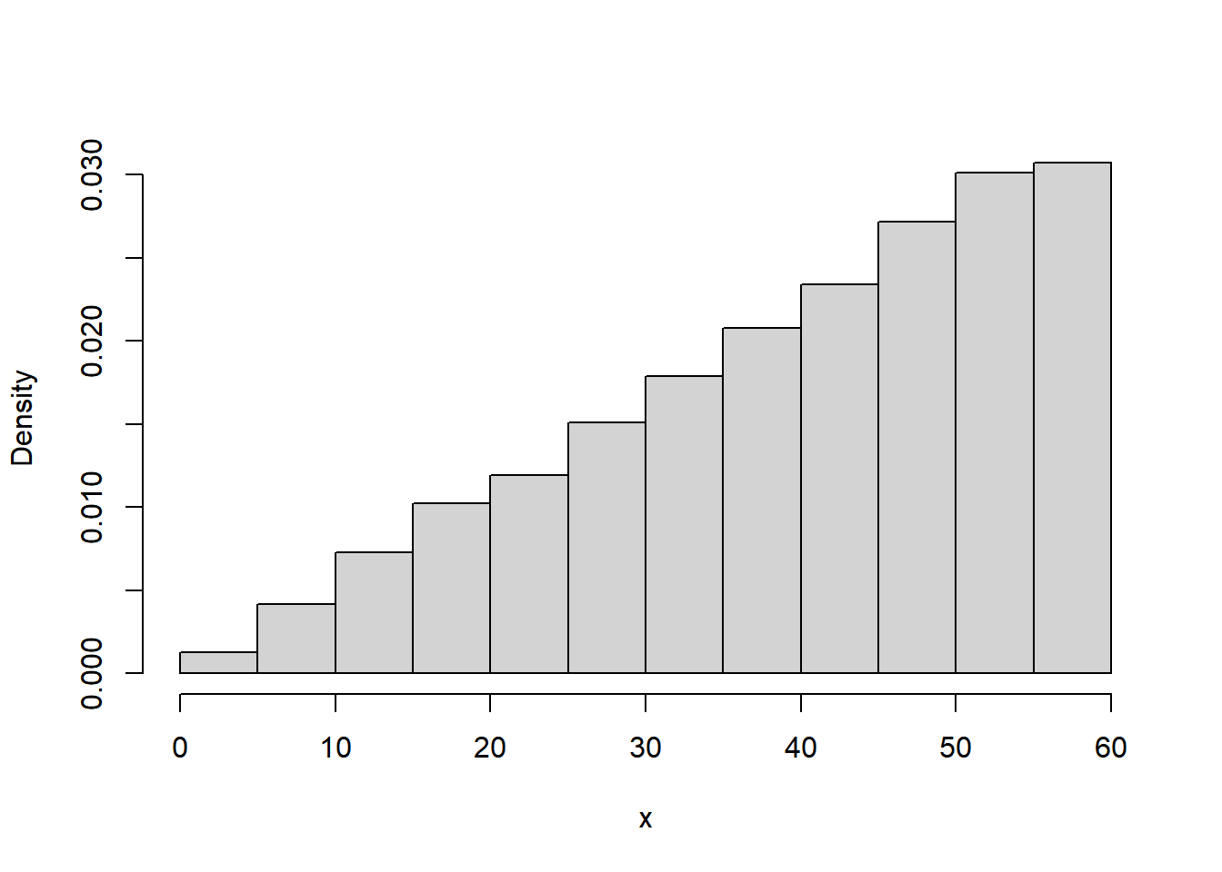

Figure 9.2: Simulated values of $X$ with the pdf in Example 9.2. (We’ll see how this simulation works soon.)

Figure 9.3: Probability of Regina arriving at each minute between noon (0) and 1:00PM (60), to the nearest minute, for the Uniform(0, 60) distribution (blue) and the distribution in Example 9.2 (orange).

• The probability that a continuous random variable $X$ equals any particular value is 0. That is, if $X$ is continuous then $\text{P}(X=x)=0$ for all $x$.
  
• For continuous random variables, it doesn’t really make sense to talk about the probability that the random value is equal to a particular value. However, we can consider the probability that a random variable is close to a particular value.
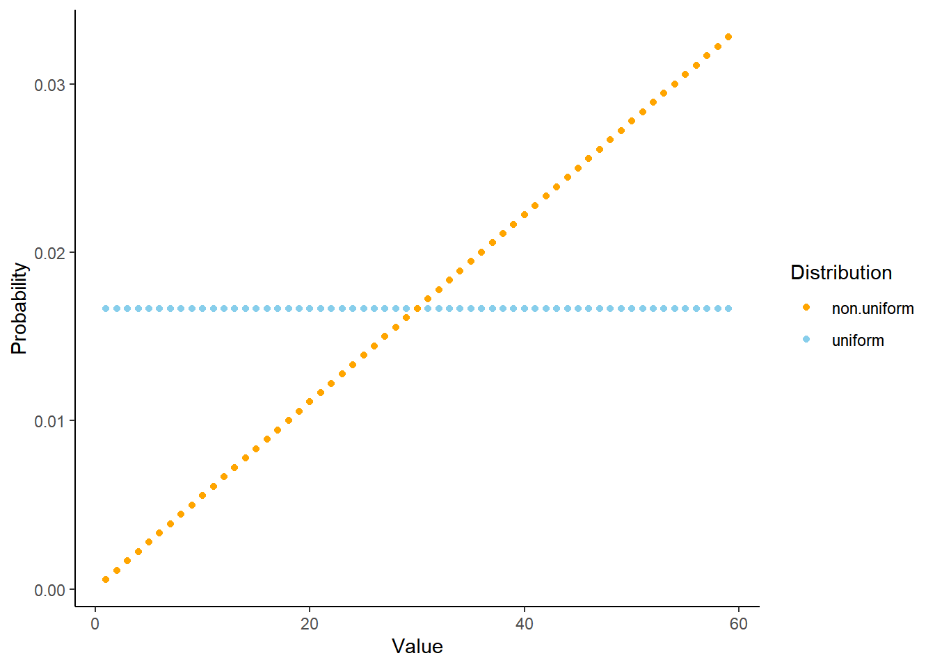
• The density $f_X(x)$ at value $x$ is not a probability.
• Rather, the density $f_X(x)$ at value $x$ is related to the probability that the RV $X$ takes a value “close to $x$” in the following sense $$\text{P}(x-\frac{ϵ}{2}\le X\le x+\frac{ϵ}{2})\approx f_X(x)ϵ,\text{for small }ϵ$$
• The quantity $ϵ$ is a small number that represents the desired degree of precision. For example, rounding to two decimal places corresponds to $ϵ=0.01$.
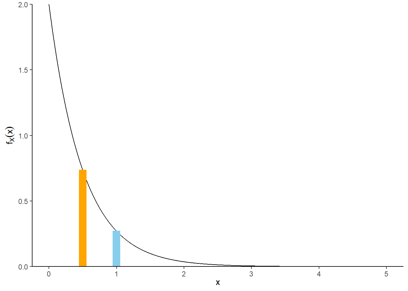
• What’s important about a pdf is relative heights. For example, if $f_X(x_2)=2f_X(x_1)$ then $X$ is roughly “twice as likely to be near $x_2$ than to be near $x_1$” in the above sense. $$\frac{f_X(x_2)}{f_X(x_1)}=\frac{f_X(x_2)ϵ}{f_X(x_1)ϵ}\approx \frac{\text{P}(x_2-\frac{ϵ}{2}\le X\le x_2+\frac{ϵ}{2})}{\text{P}(x_1-\frac{ϵ}{2}\le X\le x_1+\frac{ϵ}{2})}$$

9.3 Exponential Distributions

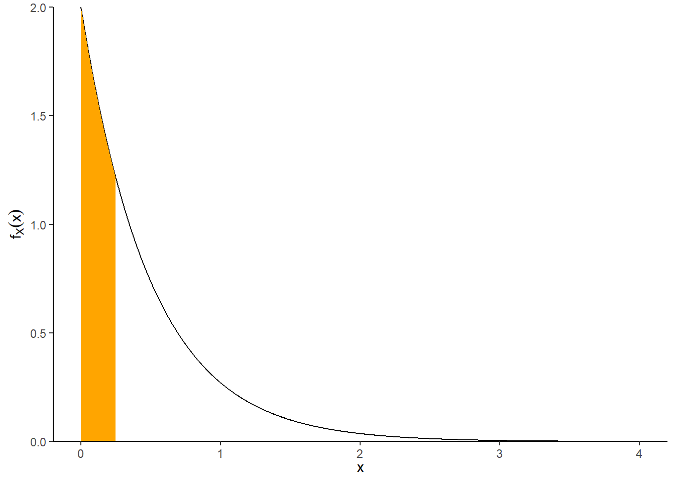
Example 9.3 Suppose that we model the waiting time, measured continuously in hours, from now until the next earthquake (of any magnitude) occurs in southern CA as a continuous random variable $X$ with pdf

$$f_X(x)=2e^{-2x},x\ge 0$$

This is the pdf of the “Exponential(2)” distribution.

1. Sketch the pdf of $X$. What does this tell you about waiting times?
   
   
   
   
   
2. Without doing any integration, approximate the probability that $X$ rounded to the nearest minute is 0.5 hours.
   
   
   
   
   
3. Without doing any integration determine how much more likely that $X$ rounded to the nearest minute is to be 0.5 than 1.0.
   
   
   
   
   
4. Compute and interpret $\text{P}(X>0.25)$.
   
   
   
   
   
5. Compute and interpret $\text{P}(X\le 3)$.
   
   
   
   
   

• A continuous random variable $X$ has an Exponential distribution with rate parameter $\lambda >0$ if its pdf is $$f_X(x)=\lambda e^{-\lambda x},x\ge 0$$
• If $X$ has an Exponential($\lambda$) distribution then $$\text{P}(X>x)=e^{-\lambda x},x\ge 0$$
• In R:
  • rexp(N_rep, rate) to simulate values
  • dexp(x, rate) to compute the probability density function
  • pexp(x, rate) to compute the cumulative distribution function $\text{P}(X\le x)$.
  • qexp(p, rate) to compute the quantile function which returns $x$ for which $\text{P}(X\le x)=p$.
• Exponential distributions are often used to model the waiting time in a random process until some event occurs.
  • $\lambda$ is the average rate at which events occur over time (e.g., 2 per hour)
  • $1/\lambda$ is the mean time between events (e.g., 1/2 hour)

N_rep = 10000

x = rexp(N_rep, rate = 2)

head(x) |>
  kbl()

x
0.4848519
0.0190915
1.3624062
0.0464219
0.4694797
0.8382753

sum(x <= 3) / N_rep

[1] 0.9975

pexp(3, 2)

[1] 0.9975212

sum(x > 0.25) / N_rep

[1] 0.6151

1 - pexp(0.25, 2)

[1] 0.6065307

hist(x,
     freq = FALSE,
     main = "",
     breaks = 20)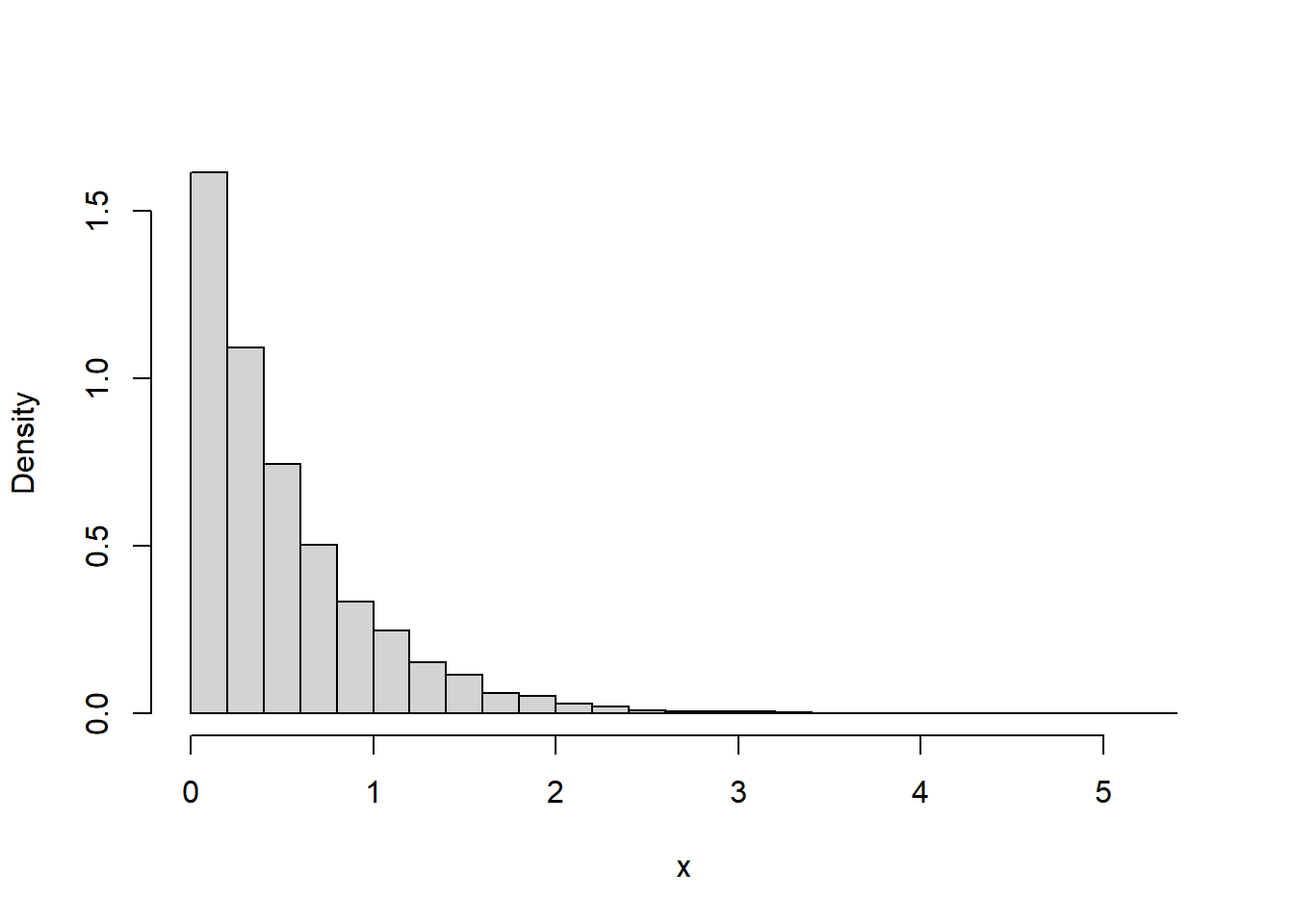

Figure 9.4: Simulated values from an Exponential distribution with rate 2.

Figure 9.5: Probability density function of $X$ with an Exponential distribution with rate 2. The shaded area represents $P(X<0.25)$.

Figure 9.6: Illustration that the probability that $X$ is close to $x$ can be approximated by the area of a rectangle with height equal to the density at $x$, $f_X(x)$. The density height at $x=0.5$ is roughly 2.7 times greater than the density height at $x=1$ so the probability that $X$ is close to 0.5 is roughly 2.7 times greater than the probability that $X$ is close to 1.

9.4 Expected Values

• The expected value (a.k.a. expectation a.k.a. mean), of a random variable $X$ is a number denoted $\text{E}(X)$ representing the probability-weighted average value of $X$.
• The expected value of a continuous random variable with pdf $f_X$ is defined as $$\text{E}(X)={\int }_{-\mathrm{\infty }}^{\mathrm{\infty }}x{f}_X(x)dx$$
• Replace the generic bounds $(-\mathrm{\infty },\mathrm{\infty })$ with the possible values of the random variable
• Note well that $\text{E}(X)$ represents a single number.
• The expected value is the “balance point” (center of gravity) of a distribution.
• The expected value of a random variable $X$ is defined by the probability-weighted average according to the underlying probability measure. But the expected value can also be interpreted as the long-run average value, and so can be approximated via simulation.
• Read the symbol $\text{E}(\cdot )$ as
  • Simulate lots of values of what’s inside $(\cdot )$
  • Compute the average. This is a “usual” average; just sum all the simulated values and divide by the number of simulated values.

Example 9.4

Continuing Example 9.3, where $X$, the waiting time (hours) from now until the next earthquake (of any magnitude) occurs in southern CA, has an Exponential distribution with rate 2.

1. Use simulation to approximate the long run average value of $X$.
   
   
   
   
2. Set up the integral to compute $\text{E}(X)$.
   
   
   
   
   
3. Interpret $\text{E}(X)$.
   
   
   
   
   
4. Compute $\text{P}(X=\text{E}(X))$.
   
   
   
   
   
5. Compute $\text{P}(X\le \text{E}(X))$. (Is it equal to 50%?)
   
   
   
   
   

sum(x) / N_rep

[1] 0.5070349

mean(x)

[1] 0.5070349

sum(x <= mean(x)) / N_rep

[1] 0.6304

pexp(0.5, 2)

[1] 0.6321206

• If $X$ has an Exponential($\lambda$) distribution then $$\text{E}(X)=\frac{1}{\lambda }$$
• For example, if events happen at rate $\lambda =2$ per hour, then the average waiting time between events is $1/\lambda =1/2$ hour.

9.5 Law of the Unconscious Statistician

• The “law of the unconscious statistician” (LOTUS) says that the expected value of a transformed random variable can be found without finding the distribution of the transformed random variable, simply by applying the probability weights of the original random variable to the transformed values. $$\begin{array}{rlrl}& \text{Discrete }X\text{ with pmf }{p}_X\text{:}& \text{E}[g(X)]& =\sum _{x}g(x)p_X(x)\\ & \text{Continuous }X\text{ with pdf }{f}_X\text{:}& \text{E}[g(X)]& ={\int }_{-\mathrm{\infty }}^{\mathrm{\infty }}g(x)f_X(x)dx\end{array}$$
• LOTUS says we don’t have to first find the distribution of $Y=g(X)$ to find $\text{E}[g(X)]$; rather, we just simply apply the transformation $g$ to each possible value $x$ of $X$ and then apply the corresponding weight for $x$ to $g(x)$.
• Whether in the short run or the long run, in general $$\begin{array}{rl}\text{Average of }g(X)& \ne g(\text{Average of }X)\end{array}$$
• In terms of expected values, in general $$\begin{array}{rl}\text{E}(g(X))& \ne g(\text{E}(X))\end{array}$$ The left side $\text{E}(g(X))$ represents first transforming the $X$ values and then averaging the transformed values. The right side $g(\text{E}(X))$ represents first averaging the $X$ values and then plugging the average (a single number) into the transformation formula.

Example 9.5

Continuing Example 9.3, where $X$, the waiting time (hours) from now until the next earthquake (of any magnitude) occurs in southern CA, has an Exponential distribution with rate 2.

1. Use simulation to approximate the variance of $X$.
   
   
   
   
2. Set up the integral to compute $\text{E}(X^2)$.
   
   
   
   
   
3. Compute $\text{Var}(X)$. (The previous part shows $\text{E}(X^2)=0.5$)
   
   
   
   
   
4. Compute $\text{SD}(X)$.
   
   
   
   
   

data.frame(x,
           x - mean(x),
           (x - mean(x)) ^ 2) |>
  head() |>
  kbl(col.names = c("Value", "Deviation from mean", "Squared deviation")) |>
  kable_styling(fixed_thead = TRUE)

Value	Deviation from mean	Squared deviation
0.4848519	-0.0221830	0.0004921
0.0190915	-0.4879434	0.2380888
1.3624062	0.8553713	0.7316601
0.0464219	-0.4606131	0.2121644
0.4694797	-0.0375553	0.0014104
0.8382753	0.3312403	0.1097202

mean(x)

[1] 0.5070349

mean((x - mean(x)) ^ 2)

[1] 0.2489758

var(x)

[1] 0.2490007

sqrt(var(x))

[1] 0.4989997

sd(x)

[1] 0.4989997

mean(x ^ 2)

[1] 0.5060602

• The variance of a random variable $X$ is $$\begin{array}{rl}\text{Var}(X)& =\text{E}\left({(X-\text{E}(X))}^2\right)\\ & =\text{E}\left(X^2\right)-{(\text{E}(X))}^2\end{array}$$
• The standard deviation of a random variable is $$\text{SD}(X)=\sqrt{\text{Var}(X)}$$
• Variance is the long run average squared deviation from the mean.
• Standard deviation measures, roughly, the long run average distance from the mean. The measurement units of the standard deviation are the same as for the random variable itself.
• The definition $\text{E}((X-\text{E}(X){)}^2)$ represents the concept of variance. However, variance is usually computed using the following equivalent but slightly simpler formula. $$\text{Var}(X)=\text{E}\left(X^2\right)-{\left(\text{E}\left(X\right)\right)}^2$$
• That is, variance is the expected value of the square of $X$ minus the square of the expected value of $X$.
  
• Variance has many nice theoretical properties. Whenever you need to compute a standard deviation, first find the variance and then take the square root at the end.
• If $X$ has an Exponential($\lambda$) distribution then $$\text{Var}(X)=\frac{1}{{\lambda }^2}$$