3 Conditional Probability

Example 3.1

Continuing Example 2.1. The probability that a randomly selected U.S. household has a pet dog is 0.47. The probability that a randomly selected U.S. household has a pet cat is 0.25. the probability that a randomly selected U.S. household has a pet dog and a pet cat is 0.15.

Compute the probability that a randomly selected U.S. household that has a pet dog also has a pet cat. Is it 0.25?
Compute the probability that a randomly selected U.S. household that does not have a pet dog has a pet cat. Is it the same as the previous part? Is it one minus the previous part?
Describe in words the probability that results from subtracting the answer to the first part from 1.

The conditional probability of event \(A\) given event \(B\), denoted \(\text{P}(A|B)\), is defined as \[ \text{P}(A|B) = \frac{\text{P}(A\cap B)}{\text{P}(B)} \]
The conditional probability \(\text{P}(A|B)\) represents how the likelihood or degree of uncertainty of event \(A\) should be updated to reflect information that event \(B\) has occurred.
Conditional probabilities are probabilities. There are analagous conditional versions of the properties of probability, e.g. \(\text{P}(A^c|B) = 1 - \text{P}(A|B)\).
In general, knowing whether or not event \(B\) occurs influences the probability of event \(A\). That is, \[ \text{In general, } \text{P}(A|B) \neq \text{P}(A) \]
Be careful: order is essential in conditioning. That is, \[ \text{In general, } \text{P}(A|B) \neq \text{P}(B|A) \]
Within the context of two events, we have joint, conditional, and marginal probabilities.
- Joint: unconditional probability involving both events, \(\text{P}(A \cap B)\).
- Conditional: conditional probability of one event given the other, \(\text{P}(A | B)\), \(\text{P}(B | A)\).
- Marginal: unconditional probability of a single event \(\text{P}(A)\), \(\text{P}(B)\).
The relationship \(\text{P}(A|B) = \text{P}(A\cap B)/\text{P}(B)\) can be stated generically as \[ \text{conditional} = \frac{\text{joint}}{\text{marginal}} \]
When dealing with probabilities (or proportions or percentages) be sure to ask “probability of what?” Thinking in fraction terms, be careful to identify the correct reference group which corresponds to the denominator.

Example 3.2 Are Americans in favor of free tuition at public colleges and universities? According to a study conducted by the Pew Research Center in January 2020

83% of Democrats are in favor of free tuition
60% of Independents are in favor of free tuition
39% of Republicans are in favor of free tuition

Also suppose that¹

32% of Americans are Democrats
42% of Americans are Independents
26% of Americans are Republicans

We’ll use this information to investigate the following questions, as well as a few others.

What is the probability that a randomly selected American is in favor of free college tuition?
What is the probability that a random selected American who is in favor of free college tuition is a Democrat?

Represent the given information using proper notation.
Construct a hypothetical two-way table of counts representing this scenario.
What is the probability that an American who is in favor of free college tuition is a Democrat? (For this and the remaining parts, in addition to computing, represent the probability with proper notation.)
What is the probability that an American who is a Democrat is in favor of free college tuition?
What is the probability that an Americans is a Democrat and in favor of free college tuition?
What is the probability that an American is in favor of free college tuition?

Rearranging the definition of conditional probability we get the Multiplication rule: the probability that two events both occur is \[ \begin{aligned} \text{P}(A \cap B) & = \text{P}(A|B)\text{P}(B)\\ & = \text{P}(B|A)\text{P}(A) \end{aligned} \]
The multiplication rule says that you should think “multiply” when you see “and”. However, be careful about what you are multiplying: to find a joint probability you need an unconditional and an appropriate conditional probability.
You can condition either on \(A\) or on \(B\), provided you have the appropriate marginal probability; often, conditioning one way is easier than the other.
Be careful: the multiplication rule does not say that \(\text{P}(A\cap B)\) is the same as \(\text{P}(A)\text{P}(B)\).

Example 3.3

Continuing Example 3.3. Explain in detail how you could conduct a simulation, using only the information provided in the set up, and how you would use the results to approximate the probabilities we computed in Example 3.3?

Conditional probabilities can be approximated by filtering (or subsetting) based on the condition
To approximate \(\text{P}(A|B)\), simulate the random phenomenon for a set number of repetitions (say 10000), discard those repetitions on which \(B\) does not occur, and compute the relative frequency of \(A\) among the remaining repetitions (on which \(B\) does occur).
Be careful! The margin of error is based on only the number of repetitions used to compute the relative frequency. So if you perform 10000 repetitions but \(B\) occurs only on 2000, then the margin of error for estimate \(\text{P}(A|B)\) is roughly on the order of \(1/\sqrt{2000} = 0.022\) (rather than \(1/\sqrt{10000} = 0.01\). Especially if \(\text{P}(B)\) is small, the margin of error could be large resulting in an imprecise estimate of \(\text{P}(A|B)\). (Advantage: not computationally intensive.)

N_rep = 10000

# initialize a data.frame for storing results
party_support = data.frame(party = character(),
                           free_tuition = character())

for (i in 1:N_rep) {
  party = sample(c("D", "I", "R"), size = 1, prob = c(0.32, 0.42, 0.26))
  if (party == "D") {
    free_tuition = sample(c("yes", "no"), size = 1, prob = c(0.83, 1 - 0.83))
  } else if (party == "I"){
    free_tuition = sample(c("yes", "no"), size = 1, prob = c(0.60, 1 - 0.60))
  } else {
    free_tuition = sample(c("yes", "no"), size = 1, prob = c(0.39, 1 - 0.39))
  }
  party_support[i, ] = c(party, free_tuition)
}

# first few rows; each row is a (party, support) pair
head(party_support)

  party free_tuition
1     I          yes
2     I          yes
3     D          yes
4     I          yes
5     I          yes
6     R          yes

# tabulate results with counts
table(party_support)

     free_tuition
party   no  yes
    D  529 2675
    I 1693 2509
    R 1612  982

# tabulate results with proportions
table(party_support) / N_rep

     free_tuition
party     no    yes
    D 0.0529 0.2675
    I 0.1693 0.2509
    R 0.1612 0.0982

# Approximate P(D and Support)
nrow(party_support[(party_support$party == "D") & (party_support$free_tuition == "yes"), ]) / N_rep

[1] 0.2675

# Approximate P(D | Support)
nrow(party_support[(party_support$party == "D") & (party_support$free_tuition == "yes"), ]) / nrow(party_support[party_support$free_tuition == "yes", ])

[1] 0.4338307

library(tidyverse)

# Counting in a different way
party_support |>
  filter(party == "D", free_tuition == "yes") |>
  count()

     n
1 2675

library(ggmosaic)

ggplot(party_support) +
  geom_mosaic(aes(x = product(free_tuition, party),
                  fill = free_tuition)) +
  theme_mosaic()

Warning: `unite_()` was deprecated in tidyr 1.2.0.
Please use `unite()` instead.
This warning is displayed once every 8 hours.
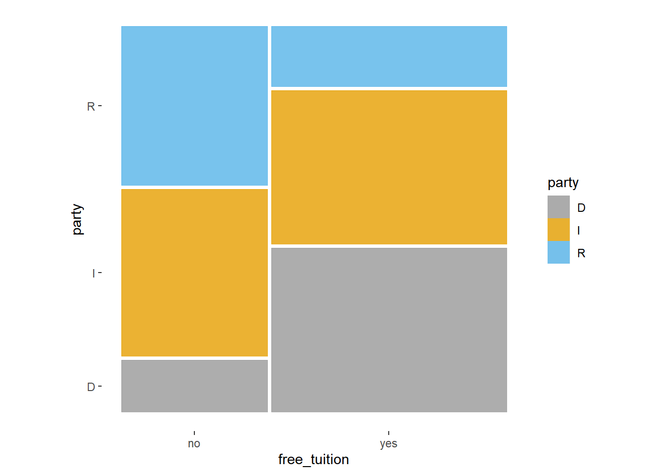
Call `lifecycle::last_lifecycle_warnings()` to see where this warning was generated.

ggplot(party_support) +
  geom_mosaic(aes(x = product(party, free_tuition),
                  fill = party)) +
  theme_mosaic()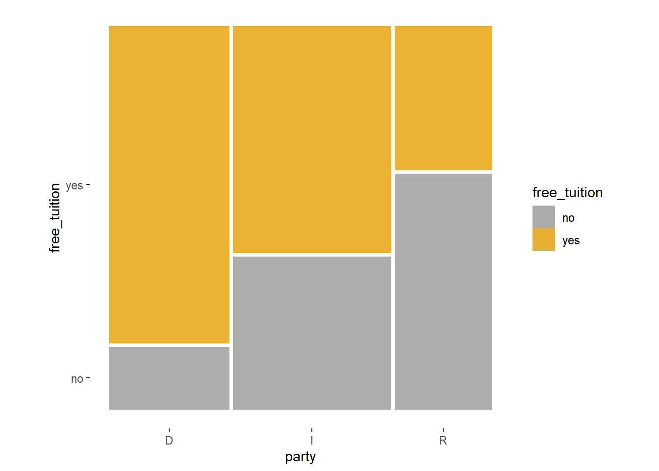

Mosaic plot of free tuition support given party

Mosaic plot of party given free tuition support

3.1 Bayes Rule

Bayes’ rule describes how to update uncertainty in light of new information, evidence, or data.

Example 3.4 A recent survey of American adults asked: “Based on what you have heard or read, which of the following two statements best describes the scientific method?”

70% selected “The scientific method produces findings meant to be continually tested and updated over time”. (We’ll call this the “iterative” opinion.)
14% selected “The scientific method identifies unchanging core principles and truths”. (We’ll call this the “unchanging” opinion).
16% were not sure which of the two statements was best.

How does the response to this question change based on education level? Suppose education level is classified as: high school or less (HS), some college but no Bachelor’s degree (college), Bachelor’s degree (Bachelor’s), or postgraduate degree (postgraduate). The education breakdown is

Among those who agree with “iterative”: 31.3% HS, 27.6% college, 22.9% Bachelor’s, and 18.2% postgraduate.
Among those who agree with “unchanging”: 38.6% HS, 31.4% college, 19.7% Bachelor’s, and 10.3% postgraduate.
Among those “not sure”: 57.3% HS, 27.2% college, 9.7% Bachelor’s, and 5.8% postgraduate

Use the information to construct an appropriate two-way table.
Overall, what percentage of adults have a postgraduate degree? How is this related to the values 18.2%, 10.3%, and 5.8%?
What percent of those with a postgraduate degree agree that the scientific method is “iterative”? How is this related to the values provided?

Bayes’ rule for events specifies how a prior probability \(P(H)\) of event \(H\) is updated in response to the evidence \(E\) to obtain the posterior probability \(P(H|E)\). \[ \text{P}(H|E) = \frac{\text{P}(E|H)\text{P}(H)}{\text{P}(E)} \]
Event \(H\) represents a particular hypothesis (or model or case)
Event \(E\) represents observed evidence (or data or information)
\(\text{P}(H)\) is the unconditional or prior probability of \(H\) (prior to observing evidence \(E\))
\(\text{P}(H|E)\) is the conditional or posterior probability of \(H\) after observing evidence \(E\).
\(\text{P}(E|H)\) is the likelihood of evidence \(E\) given hypothesis (or model or case) \(H\)

Example 3.5

Continuing the previous example. Randomly select an American adult.

Consider the conditional probability that a randomly selected American adult agrees that the scientific method is “iterative” given that they have a postgraduate degree. Identify the prior probability, hypothesis, evidence, likelihood, and posterior probability, and use Bayes’ rule to compute the posterior probability.
Find the conditional probability that a randomly selected American adult with a postgraduate degree agrees that the scientific method is “unchanging”.
Find the conditional probability that a randomly selected American adult with a postgraduate degree is not sure about which statement is best.
How many times more likely is it for an American adult to have a postgraduate degree and agree with the “iterative” statement than to have a postgraduate degree and agree with the “unchanging” statement?
How many times more likely is it for an American adult with a postgraduate degree to agree with the “iterative” statement than to agree with the “unchanging” statement?
What do you notice about the answers to the two previous parts?
How many times more likely is it for an American adult to agree with the “iterative” statement than to agree with the “unchanging” statement?
How many times more likely is it for an American adult to have a postgraduate degree when the adult agrees with the iterative statement than when the adult agree with the unchanging statement?
How many times more likely is it for an American adult with a postgraduate degree to agree with the “iterative” statement than to agree with the “unchanging” statement?
How are the values in the three previous parts related?

Bayes rule is often used when there are multiple hypotheses or cases. Suppose \(H_1,\ldots, H_k\) is a series of distinct hypotheses which together account for all possibilities, and \(E\) is any event (evidence).
Combining Bayes’ rule with the law of total probability, \[\begin{align*} P(H_j |E) & = \frac{P(E|H_j)P(H_j)}{P(E)}\\ & = \frac{P(E|H_j)P(H_j)}{\sum_{i=1}^k P(E|H_i) P(H_i)}\\ & \\ P(H_j |E) & \propto P(E|H_j)P(H_j) \end{align*}\]
The symbol \(\propto\) is read “is proportional to”. The relative ratios of the posterior probabilities of different hypotheses are determined by the product of the prior probabilities and the likelihoods, \(P(E|H_j)P(H_j)\). The marginal probability of the evidence, \(P(E)\), in the denominator simply normalizes the numerators to ensure that the updated probabilities sum to 1 over all the distinct hypotheses.
In short, Bayes’ rule says \[ \textbf{posterior} \propto \textbf{likelihood} \times \textbf{prior} \]

Example 3.6

Now suppose we want to compute the posterior probabilities for an American adult’s perception of the scientific method given that the randomly selected American adult has some college but no Bachelor’s degree (“college”).

Before computing, make an educated guess for the posterior probabilities. In particular, will the changes from prior to posterior be more or less extreme given the American has some college but no Bachelor’s degree than when given the American has a postgraduate degree? Why?
Construct a Bayes table and compute the posterior probabilities. Compare to the posterior probabilities given postgraduate degree from the previous examples.

Bayesian analysis is often an iterative process.
Posterior probabilities are updated after observing some information or data. These probabilities can then be used as prior probabilities before observing new data.
Posterior probabilities can be sequentially updated as new data becomes available, with the posterior probabilities after the previous stage serving as the prior probabilities for the next stage.
The final posterior probabilities only depend upon the cumulative data. It doesn’t matter if we sequentially update the posterior after each new piece of data or only once after all the data is available; the final posterior probabilities will be the same either way. Also, the final posterior probabilities are not impacted by the order in which the data are observed.

These values are based on surveys by Gallup, but the values change somewhat over time.↩︎