11  Normal Distributions

• Normal distributions are probably the most important distributions in probability and statistics.
• A continuous random variable \(X\) has a Normal (a.k.a., Gaussian) distribution with mean \(\mu\in (-\infty,\infty)\) and standard deviation \(\sigma>0\) if its pdf is \[ f_X(x) = \frac{1}{\sigma\sqrt{2\pi}}\,\exp\left(-\frac{1}{2}\left(\frac{x-\mu}{\sigma}\right)^2\right), \quad -\infty<x<\infty \]
• If \(X\) has a Normal(\(\mu\), \(\sigma\)) distribution then \[\begin{align*} \text{E}(X) & = \mu\\ \text{SD}(X) & = \sigma \end{align*}\]
• In R:
  • rnorm(N_rep, mean, sd) to simulate values
  • dnorm(x, mean, sd) to compute the probability density function
  • pnorm(x, mean, sd) to compute the cumulative distribution function \(\text{P}(X \le x)\).
  • qnorm(p, mean, sd) to compute the quantile function which returns \(x\) for which \(\text{P}(X\le x) = p\).
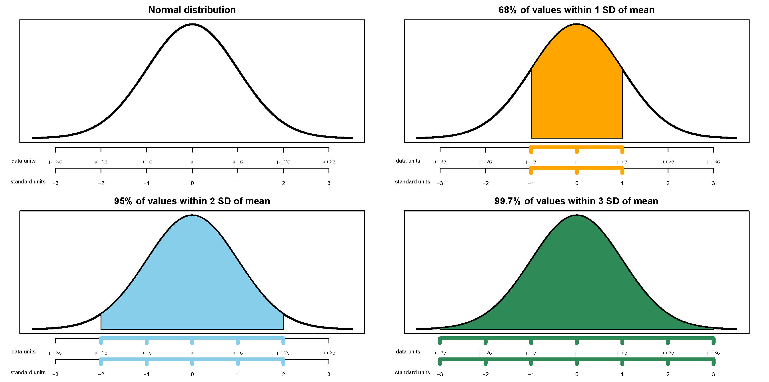
• A Normal density is a particular “bell-shaped” curve which is symmetric about its mean \(\mu\). The mean \(\mu\) is a location parameter: \(\mu\) indicates where the center and peak of the distribution is.
• The standard deviation \(\sigma\) is a scale parameter: \(\sigma\) indicates the distance from the mean to where the concavity of the density changes. That is, there are inflection points at \(\mu\pm \sigma\).

Example 11.1

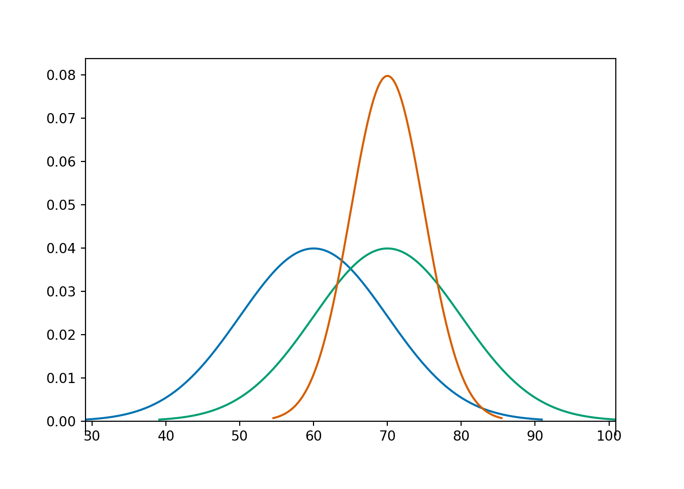
The pdfs in the plot below represent the distribution of hypothetical test scores in three classes. The test scores in each class follow a Normal distribution. Identify the mean and standard deviation for each class.

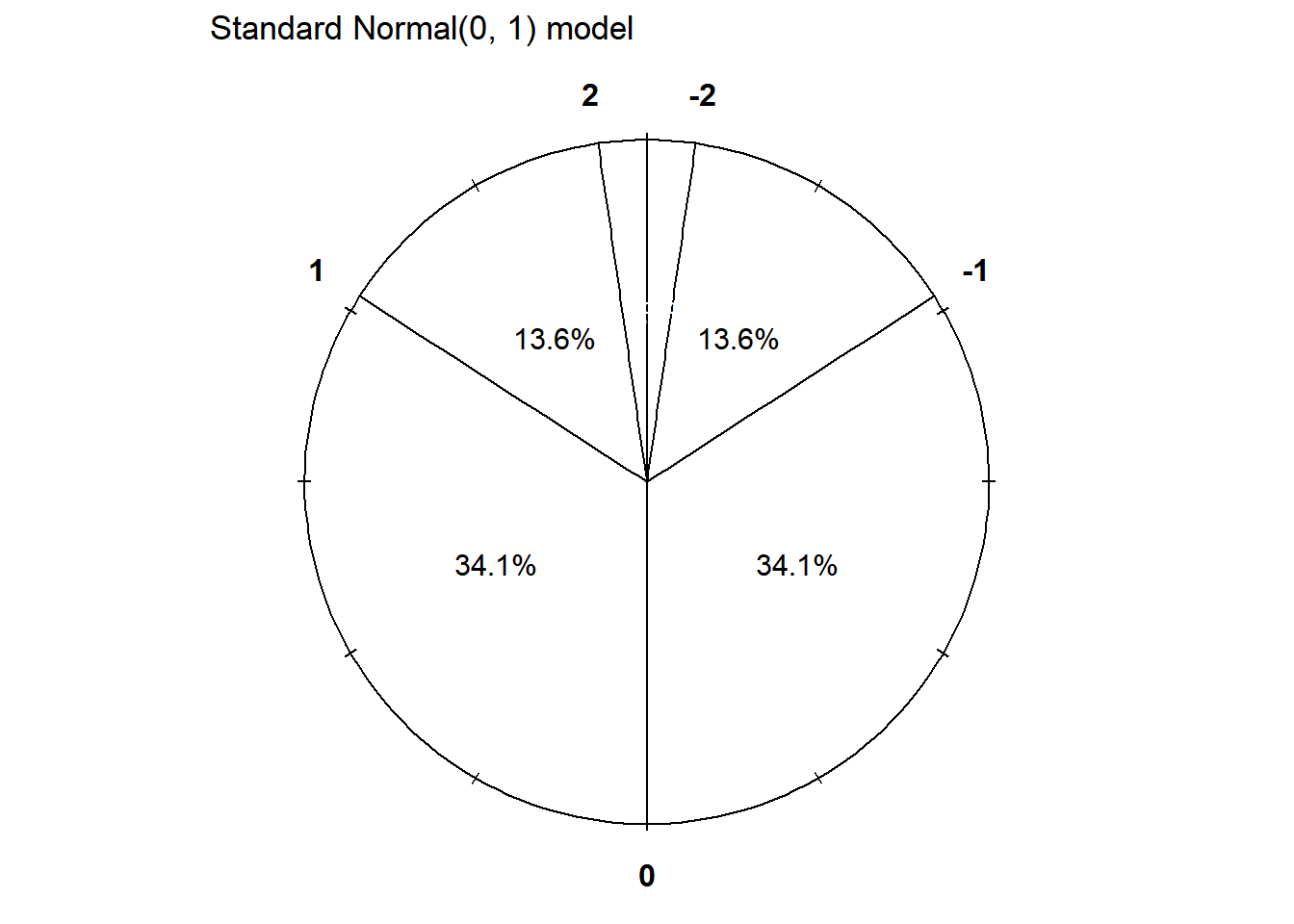
• Any Normal distribution follows the “empirical rule” which determines the percentiles that give a Normal distribution its particular bell shape.
• For a Normal distribution:
  • 38% of values are within 0.5 standard deviations of the mean
  • 68% of values are within 1 standard deviation of the mean
  • 87% of values are within 0.5 standard deviations of the mean
  • 95% of values are within 2 standard deviations of the mean
  • 99% of values are within 2.6 standard deviations of the mean
  • 99.7% of values are within 3 standard deviations of the mean
• The table below lists some percentiles of a Normal distribution.

Table 11.1: Selected percentiles for a Normal distribution

Percentile	SDs away from the mean
0.1%	3.09 SDs below the mean
0.5%	2.58 SDs below the mean
1%	2.33 SDs below the mean
2.5%	1.96 SDs below the mean
10%	1.28 SDs below the mean
15.9%	1 SDs below the mean
25%	0.67 SDs below the mean
30.9%	0.5 SDs below the mean
50%	0 SDs above the mean
69.1%	0.5 SDs above the mean
75%	0.67 SDs above the mean
84.1%	1 SDs above the mean
90%	1.28 SDs above the mean
97.5%	1.96 SDs above the mean
99%	2.33 SDs above the mean
99.5%	2.58 SDs above the mean
99.9%	3.09 SDs above the mean

Figure 11.1: A standard Normal(0, 1) spinner. The same spinner is displayed on both sides, with different features highlighted on the left and right. Only selected rounded values are displayed, but in the idealized model the spinner is infinitely precise so that any real number is a possible outcome. Notice that the values on the axis are not evenly spaced.

Figure 11.2: A standard Normal(0, 1) spinner. The same spinner is displayed on both sides, with different features highlighted on the left and right. Only selected rounded values are displayed, but in the idealized model the spinner is infinitely precise so that any real number is a possible outcome. Notice that the values on the axis are not evenly spaced.

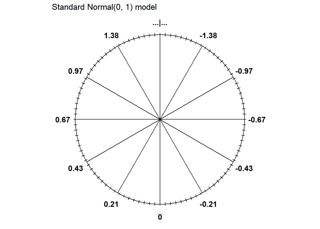
• The Normal(0, 1) distribution (mean 0, SD 1) is called the “Standard Normal” distribution
• Standardization:
  • If \(X\) has a Normal(\(\mu\), \(\sigma\)) distribution then \(Z = \frac{X-\mu}{\sigma}\) has a Normal(0, 1) distribution
  • If \(Z\) has a Normal(0, 1) distribution then \(X = \mu + \sigma Z\) has a Normal(\(\mu\), \(\sigma\)) distribution

Example 11.2

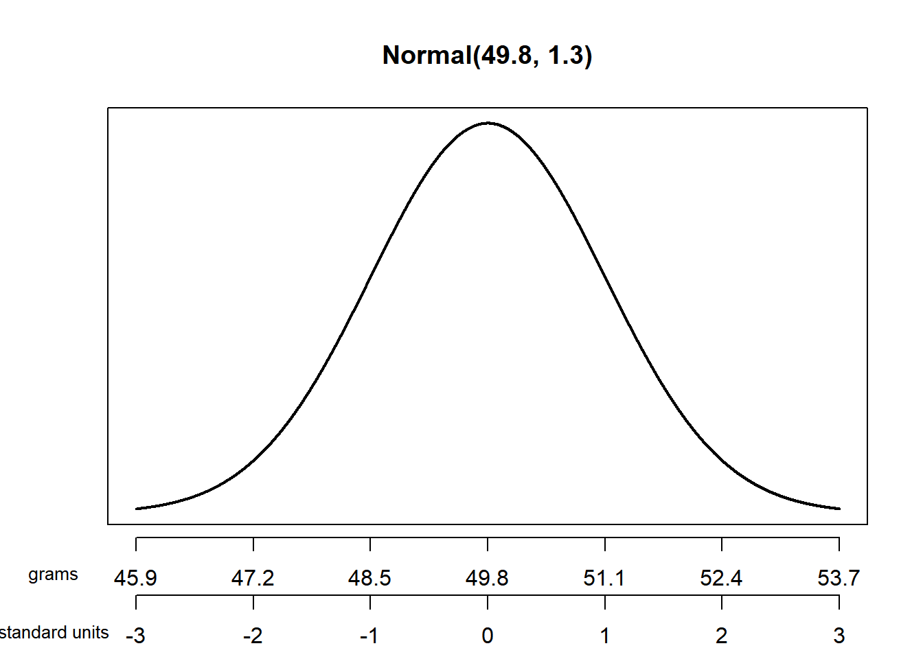
The wrapper of a package of candy lists a weight of 47.9 grams. Naturally, the weights of individual packages vary somewhat. Suppose package weights have an approximate Normal distribution with a mean of 49.8 grams and a standard deviation of 1.3 grams.

1. Sketch the distribution of package weights. Carefully label the variable axis. It is helpful to draw two axes: one in the measurement units of the variable, and one in standardized units.
   
   
   
   
   
2. Why wouldn’t the company print the mean weight of 49.8 grams as the weight on the package?
   
   
   
   
   
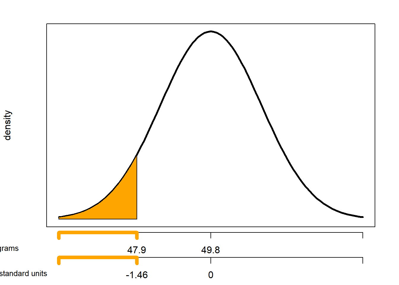
3. Estimate the probability that a package weighs less than the printed weight of 47.9 grams.
   
   
   
   
   
4. Estimate the probability that a package weighs between 47.9 and 53.0 grams.
   
   
   
   
   
5. Suppose that the company only wants 1% of packages to be underweight. Find the weight that must be printed on the packages.
   
   
   
   
   
6. Find the 25th percentile (a.k.a., first (lower) quartile) of package weights.
   
   
   
   
   
7. Find the 75th percentile (a.k.a., third (upper) quartile) of package weights. How can you use the work you did in the previous part?
   
   
   
   
   

N_rep = 10000

x = rnorm(N_rep, mean = 49.8, sd = 1.3)

head(x) |>
  kbl()

x
47.06557
49.33461
50.18085
48.88731
47.61983
51.01540

hist(x,
     freq = FALSE,
     main = "")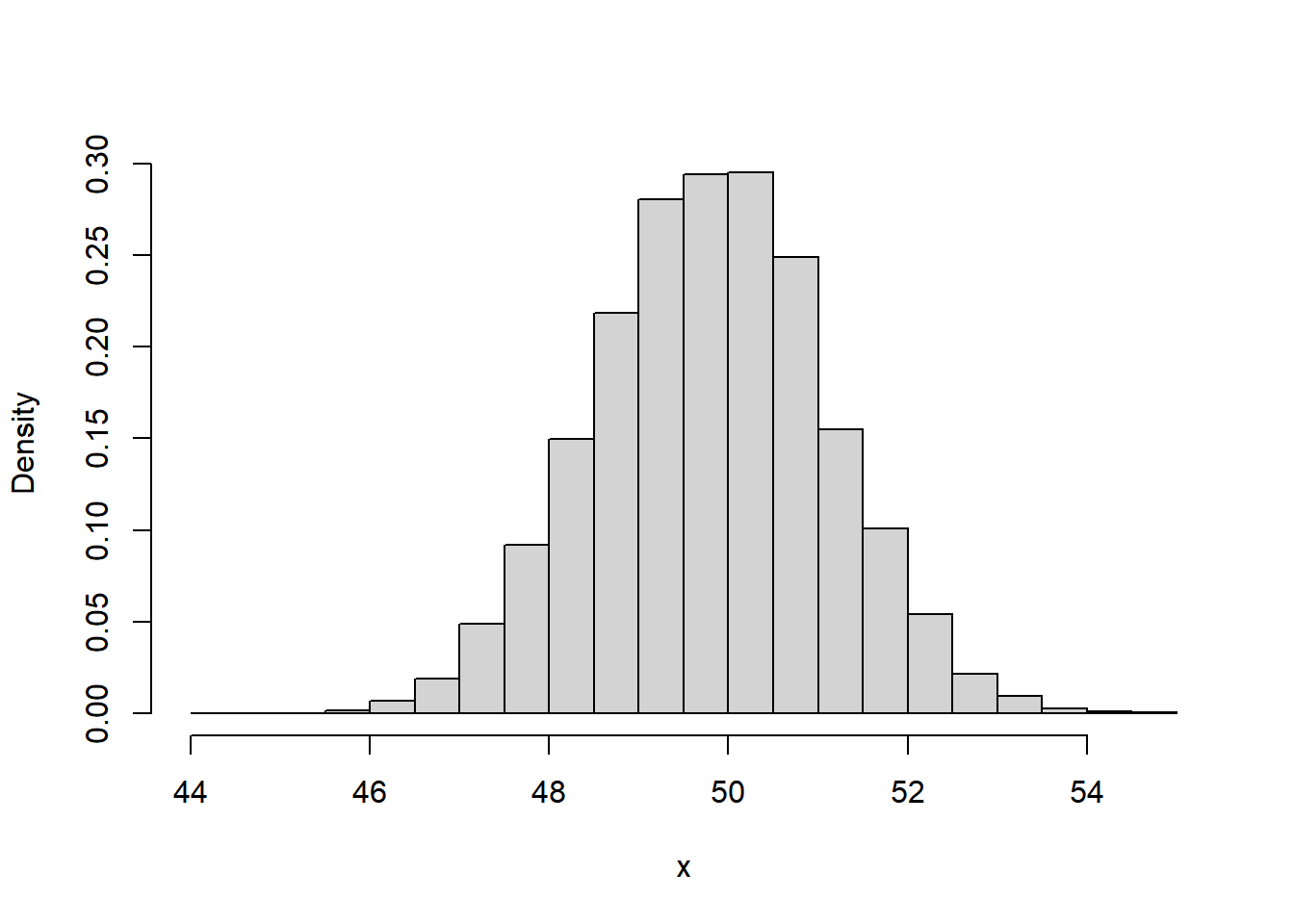

sum(x < 47.9) / N_rep

[1] 0.0721

pnorm(47.9, 49.8, 1.3)

[1] 0.07193386

pnorm((47.9 - 49.8) / 1.3)

[1] 0.07193386

sum((x > 47.9) & (x < 53))  / N_rep

[1] 0.921

pnorm(53, 49.8, 1.3) - pnorm(47.9, 49.8, 1.3)

[1] 0.921149

quantile(x, 0.01)

      1% 
46.83199 

qnorm(0.01, 49.8, 1.3)

[1] 46.77575

qnorm(0.01)

[1] -2.326348

49.8 + 1.3 * qnorm(0.01)

[1] 46.77575

Example 11.3

Daily high temperatures (degrees Fahrenheit) in San Luis Obispo in August follow (approximately) A Normal distribution with a mean of 76.9 degrees F. The temperature exceeds 100 degrees Fahrenheit on about 1.5% of August days.

1. What is the standard deviation?
   
   
   
   
   
2. Suppose the mean increases by 2 degrees Fahrenheit. On what percentage of August days will the daily high temperature exceed 100 degrees Fahrenheit? (Assume the standard deviation does not change.)
   
   
   
   
   
3. A mean of 78.9 is 1.02 times greater than a mean of 76.9. By what (multiplicative) factor has the percentage of 100-degree days increased? What do you notice?
   
   
   
   
   

Example 11.4 In a large class, scores on midterm 1 follow (approximately) a Normal\((\mu_1, \sigma)\) distribution and scores on midterm 2 follow (approximately) a Normal\((\mu_2, \sigma)\) distribution. Note that the SD \(\sigma\) is the same on both exams. The 40th percentile of midterm 1 scores is equal to the 70th percentile of midterm 2 scores. Compute

\[ \frac{\mu_1-\mu_2}{\sigma} \]

(This is one statistical measure of effect size.)