14  Conditional Distributions

• The joint distribution of random variables $X$ and $Y$ is a probability distribution on $(x,y)$ pairs, and describes how the values of $X$ and $Y$ vary together or jointly.
• We can also study conditional distributions of random variables given the values of some random variables. How does the distribution of $Y$ change for different values of $X$ (and vice versa)?

Example 14.1

Roll a fair four-sided die twice. Let $X$ be the sum of the two rolls, and let $Y$ be the larger of the two rolls (or the common value if a tie). We have previously found the joint and marginal distributions of $X$ and $Y$, displayed in the two-way table below.

$p_{X,Y}(x,y)$
$x$ \ $y$	1	2	3	4	$p_X(x)$
2	1/16	0	0	0	1/16
3	0	2/16	0	0	2/16
4	0	1/16	2/16	0	3/16
5	0	0	2/16	2/16	4/16
6	0	0	1/16	2/16	3/16
7	0	0	0	2/16	2/16
8	0	0	0	1/16	1/16
$p_Y(y)$	1/16	3/16	5/16	7/16

1. Compute $p_{X|Y}(6|4)=\text{P}(X=6|Y=4)$.
   
   
   
   
   
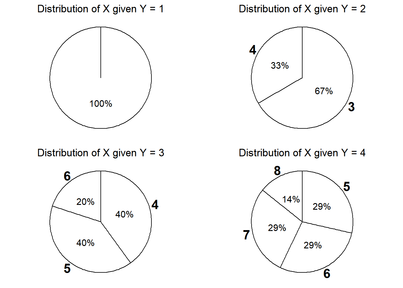
2. Construct a table, plot, and spinner to represent the conditional distribution of $X$ given $Y=4$.
   
   
   
   
   
3. Construct a table, plot, and spinner to represent the conditional distribution of $X$ given $Y=3$.
   
   
   
   
   
4. Construct a table, plot, and spinner to represent the conditional distribution of $X$ given $Y=2$.
   
   
   
   
   
5. Construct a table, plot, and spinner to represent the conditional distribution of $X$ given $Y=1$.
   
   
   
   
   
6. Compute $p_{Y|X}(4|6)=\text{P}(Y=4|X=6)$.
   
   
   
   
   
7. Construct a table, plot, and spinner to represent the distribution of $Y$ given $X=6$.
   
   
   
   
   
8. Construct a table, plot, and spinner to represent the distribution of $Y$ given $X=5$.
   
   
   
   
   
9. Construct a table, plot, and spinner to represent the distribution of $Y$ given $X=4$.
   
   
   
   
   

• The conditional distribution of $Y$ given $X=x$ is the distribution of $Y$ values over only those outcomes for which $X=x$. It is a distribution on values of $Y$ only; treat $x$ as a fixed constant when conditioning on the event $\{X=x\}$.
• Conditional distributions can be obtained from a joint distribution by slicing and renormalizing. The conditional distribution of $Y$ given $X=x$, where $x$ represents a particular number, can be thought of as:
  • the slice of the joint distribution corresponding to $X=x$, a distribution on values of $Y$ alone with $X=x$ fixed
  • renormalized so that the slice accounts for 100% of the probability over the values of $Y$
• The shape of the conditional distribution of $Y$ given $X=$ is determined by the shape of the slice of the joint distribution over values of $Y$ for the fixed $x$.
• For each fixed $x$, the conditional distribution of $Y$ given $X=x$ is a different distribution on values of the random variable $Y$. There is not one “conditional distribution of $Y$ given $X$”, but rather a family of conditional distributions of $Y$ given different values of $X$.
• Each conditional distribution is a distribution, so we can summarize its characteristics like mean and standard deviation. The conditional mean and standard deviation of $Y$ given $X=x$ represent, respectively, the long run average and variability of values of $Y$ over only $(X,Y)$ pairs with $X=x$.
• Since each value of $x$ typically corresponds to a different conditional distribution of $Y$ given $X=x$, the conditional mean and standard deviation will typically be functions of $x$.

Warning: The labeller API has been updated. Labellers taking `variable` and
`value` arguments are now deprecated. See labellers documentation.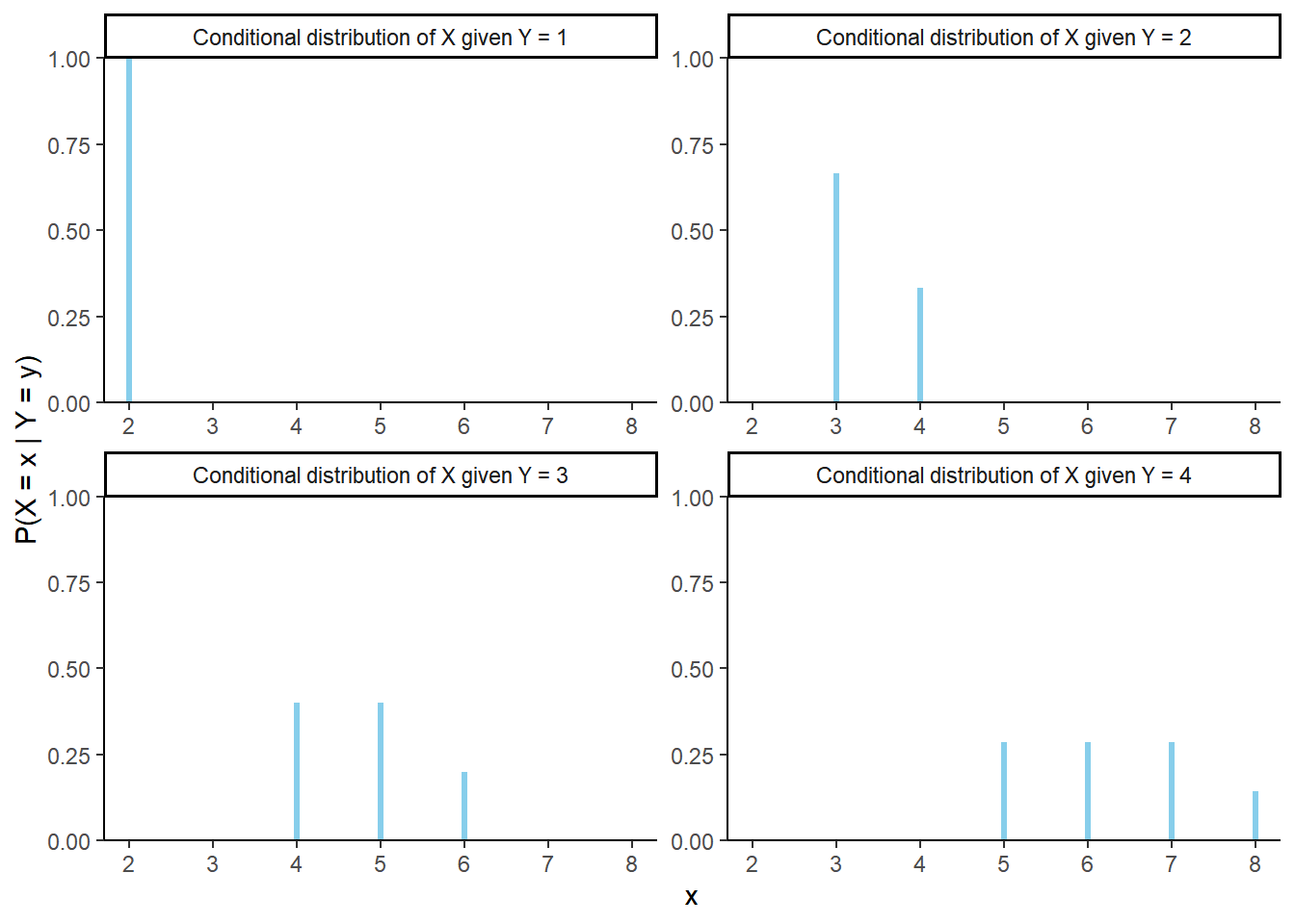

Figure 14.1: Impulse plots representing the family of conditional distributions of $X$ given $Y$ for the dice rolling example. Each plot represents a conditional distribution of $X$ given $Y=y$ for a particular value of $y=1,2,3,4$.

Figure 14.2: Spinners representing the family of conditional distributions of $X$ given $Y$ in the dice rolling example. Each spinner represents a conditional distribution of $X$ given $Y=y$ for a particular value of $y=1,2,3,4$.

Example 14.2

We have already discussed two ways for simulating an $(X,Y)$ pair in the dice rolling example: simulate a pair of rolls and measure $X$ (sum) and $Y$ (max), or spin the joint distribution spinner for $(X,Y)$ once.

1. Now describe another way for simulating an $(X,Y)$ pair using the spinners in Example 14.1. (Hint: you’ll need one more spinner in addition to the four from the previous example.)
   
   
   
   
   
2. Describe in detail how you can simulate $(X,Y)$ pairs and use the results to approximate $\text{P}(X=6|Y=4)$.
   
   
   
   
   
3. Describe in detail how you can simulate $(X,Y)$ pairs and use the results to approximate the conditional distribution of $X$ given $Y=4$.
   
   
   
   
   
4. Describe in detail how you can simulate values from the conditional distribution of $X$ given $Y=4$ without simulating $(X,Y)$ pairs.
   
   
   
   
   

• Rather than directly simulating from a joint distribution, we can simulate an $(X,Y)$ pair in two stages:
  • Simulate a value of $X$ from its marginal distribution. Call the simulated value $x$.
  • Given $x$, simulate a value of $Y$ from the conditional distribution of $Y$ given $X=x$. There will be a different distribution (spinner) for each possible value of $x$.
• This “marginal then conditional” process is essentially implementing the multiplication rule $$\text{joint}=\text{conditional}\times \text{marginal}$$
• In many problems a joint distribution is nsturally described by specifying the marginal distribution of $X$ and the family of conditional distributions of $Y$ given values of $X$

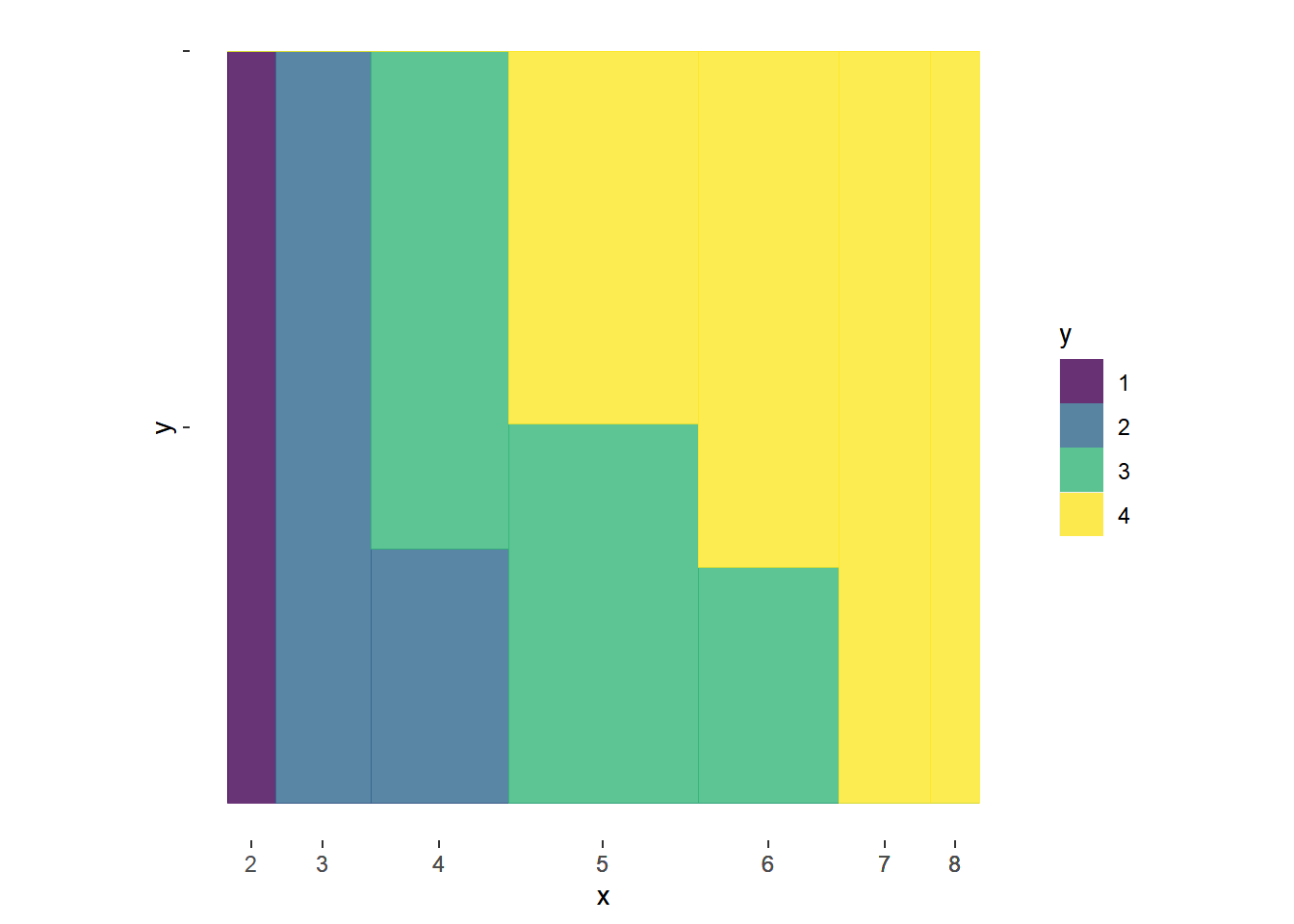
(ref:cap-dice-mosaic) Mosaic plots for Example @ref(exm:dice-conditional), where $X$ is the sum and $Y$ is the max of two rolls of a fair four-sided die. The plot on the left represents conditioning on values of the sum $X$; color represents values of $Y$. The plot on the right represents conditioning on values of the max $Y$; color represents values of $X$.

N_rep = 16000

# first roll 
u1 = sample(1:4, size = N_rep, replace = TRUE)

# second roll
u2 = sample(1:4, size = N_rep, replace = TRUE)

# sum
x = u1 + u2

# max
y = pmax(u1, u2)

dice_sim = data.frame(1:N_rep, u1, u2, x, y)

dice_sim |>
  head() |>
  kbl(col.names = c("Repetition", "First roll", "Second roll", "X (sum)", "Y (max)")) |>
  kable_styling(fixed_thead = TRUE) |>
    row_spec(which(head(y) == 4), bold = TRUE, color = "white", background = "#FFA500")

Repetition	First roll	Second roll	X (sum)	Y (max)
1	1	2	3	2
2	2	4	6	4
3	1	3	4	3
4	4	2	6	4
5	4	3	7	4
6	2	1	3	2

# Joint distribution: counts
table(x, y)

   y
x      1    2    3    4
  2 1018    0    0    0
  3    0 2025    0    0
  4    0  990 1937    0
  5    0    0 2040 2005
  6    0    0  942 2056
  7    0    0    0 1944
  8    0    0    0 1043

# Joint distribution: proportions
table(x, y) / N_rep

   y
x           1         2         3         4
  2 0.0636250 0.0000000 0.0000000 0.0000000
  3 0.0000000 0.1265625 0.0000000 0.0000000
  4 0.0000000 0.0618750 0.1210625 0.0000000
  5 0.0000000 0.0000000 0.1275000 0.1253125
  6 0.0000000 0.0000000 0.0588750 0.1285000
  7 0.0000000 0.0000000 0.0000000 0.1215000
  8 0.0000000 0.0000000 0.0000000 0.0651875

# Conditional distribution of X given Y = 4: counts
table(x[y == 4])

   5    6    7    8 
2005 2056 1944 1043 

# Conditional distribution of X given Y = 4: proportions
table(x[y == 4]) / sum(y == 4)

        5         6         7         8 
0.2844779 0.2917140 0.2758229 0.1479852 

ggplot(dice_sim) +
  geom_mosaic(aes(x = product(x, y),
                  fill = x),
              offset = 0) +
  scale_fill_viridis(discrete = TRUE) +
  theme_mosaic() +
  theme(axis.text.y=element_blank())

Warning: `unite_()` was deprecated in tidyr 1.2.0.
Please use `unite()` instead.
This warning is displayed once every 8 hours.
Call `lifecycle::last_lifecycle_warnings()` to see where this warning was generated.

ggplot(dice_sim) +
  geom_mosaic(aes(x = product(y, x),
                  fill = y),
              offset = 0) +
  scale_fill_viridis(discrete = TRUE) +
  theme_mosaic() +
  theme(axis.text.y=element_blank())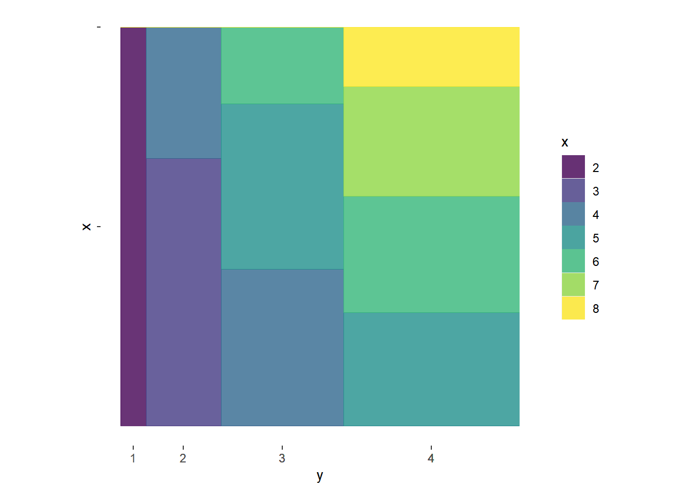

Mosaic plot of conditional distributions of X given values of Y

Mosaic plot of conditional distributions of Y given values of X

• Be sure to distinguish between joint, conditional, and marginal distributions.

• The joint distribution of $X$ and $Y$ is a distribution on $(X,Y)$ pairs. A mathematical expression of a joint distribution is a function of both values of $X$ and values of $Y$.

• The conditional distribution of $Y$ given $X=x$ is a distribution on $Y$ values (among $(X,Y)$ pairs with a fixed value of $X=x$). A mathematical expression of a conditional distribution will involve both $x$ and $y$, but $x$ is treated like a fixed constant and $y$ is treated as the variable. Note: the possible values of $Y$ might depend on the value of $x$.

• The marginal distribution of $Y$ is a distribution on $Y$ values only, regardless of the value of $X$. A mathematical expression of a marginal distribution will have only values of the single variable in it; for example, an expression for the marginal distribution of $Y$ will only have $y$ in it (no $x$, not even in the possible values).

• Be careful when conditioning with continuous random variables. Remember that the probability that a continuous random variable is equal to a particular value is 0; that is, for continuous $X$, $\text{P}(X=x)=0$. - Mathematically, when we condition on $\{X=x\}$ we are really conditioning on $\{|X-x|<ϵ\}$ — the event that the random variable $X$ is within $ϵ$ of the value $x$ — and seeing what happens in the idealized limit when $ϵ\to 0$.

• Practically, $ϵ$ represents our “close enough” degree of precision, e.g., $ϵ=0.01$ if “within 0.01” is close enough.

• When conditioning on a continuous random variable $X$ in a simulation, never condition on $\{X=x\}$; rather, condition on $\{|X-x|<ϵ\}$ where $ϵ$ represents the suitable degree of precision.

14.1 Conditional Expected Value

Example 14.3

Roll a fair four-sided die twice. Let $X$ be the sum of the two rolls, and let $Y$ be the larger of the two rolls (or the common value if a tie).

$p_{X,Y}(x,y)$
$x$ \ $y$	1	2	3	4	$p_X(x)$
2	1/16	0	0	0	1/16
3	0	2/16	0	0	2/16
4	0	1/16	2/16	0	3/16
5	0	0	2/16	2/16	4/16
6	0	0	1/16	2/16	3/16
7	0	0	0	2/16	2/16
8	0	0	0	1/16	1/16
$p_Y(y)$	1/16	3/16	5/16	7/16

1. Compute and interpret $\text{E}(Y)$. How could you find a simulation-based approximation?
   
   
   
2. We have seen that the long run average value of $Y$ is 3.125. Would you expect the conditional long run average value of $Y$ given $X=8$ to be greater than, less than, or equal to 3.125? Explain without doing any calculations. What about given $Y=3$?
   
   
   
   
   
3. How could you use simulation to approximate the conditional long run average value of $Y$ given $X=6$?
   
   
   
   
   
4. Compute and interpret $\text{E}(Y|X=6)$.
   
   
   
5. Find $\text{E}(Y|X=x)$ for each possible value of $x$ of $X$.
   
   
   
   
   
6. Compute and interpret $\text{E}(X|Y=4)$. How could you find a simulation-based approximation?
   
   
   
7. Find $\text{E}(X|Y=y)$ for each possible value $y$ of $Y$.
   
   
   
   
   

• The conditional expected value (a.k.a. conditional expectation a.k.a. conditional mean), of a random variable $Y$ given the event $\{X=x\}$, defined on a probability space with measure $\text{P}$, is a number denoted $\text{E}(Y|X=x)$ representing the probability-weighted average value of $Y$, where the weights are determined by the conditional distribution of $Y$ given $X=x$. $$\begin{array}{rlrl}& \text{Discrete }X,Y\text{ with conditional pmf }{p}_{Y|X}\text{:}& \text{E}(Y|X=x)& =\sum _{y}y{p}_{Y|X}(y|x)\end{array}$$
• Remember, when conditioning on $X=x$, $x$ is treated as a fixed constant. The conditional expected value $\text{E}(Y|X=x)$ is a number representing the mean of the conditional distribution of $Y$ given $X=x$.
• The conditional expected value $\text{E}(Y|X=x)$ is the long run average value of $Y$ over only those outcomes for which $X=x$.
• To approximate $\text{E}(Y|X=x)$, simulate many $(X,Y)$ pairs, discard the pairs for which $X\ne x$, and average the $Y$ values for the pairs that remain.

# Approximate E(Y)
mean(y)

[1] 3.124812

# Approximate E(Y| X = 6)

mean(y[x == 6])

[1] 3.685791