15  Joint Normal Distributions

• Jointly continuous random variables \(X\) and \(Y\) have a Bivariate Normal distribution with parameters \(\mu_X\), \(\mu_Y\), \(\sigma_X>0\), \(\sigma_Y>0\), and \(-1<\rho<1\) if the joint pdf is { \[\begin{align*} f_{X, Y}(x,y) & = \frac{1}{2\pi\sigma_X\sigma_Y\sqrt{1-\rho^2}}\exp\left(-\frac{1}{2(1-\rho^2)}\left[\left(\frac{x-\mu_X}{\sigma_X}\right)^2+\left(\frac{y-\mu_Y}{\sigma_Y}\right)^2-2\rho\left(\frac{x-\mu_X}{\sigma_X}\right)\left(\frac{y-\mu_Y}{\sigma_Y}\right)\right]\right) \end{align*}\] }
• If the pair \((X, Y)\) has a BivariateNormal(\(\mu_X\), \(\mu_Y\), \(\sigma_X\), \(\sigma_Y\), \(\rho\)) distribution \[\begin{align*} \text{E}(X) & =\mu_X\\ \text{E}(Y) & =\mu_Y\\ \text{SD}(X) & = \sigma_X\\ \text{SD}(Y) & = \sigma_Y\\ \text{Corr}(X, Y) & = \rho \end{align*}\]

Figure 15.1: Bivariate Normal distribution with means (0, 0), standard deviations (1, 1) and correlation 0.7.

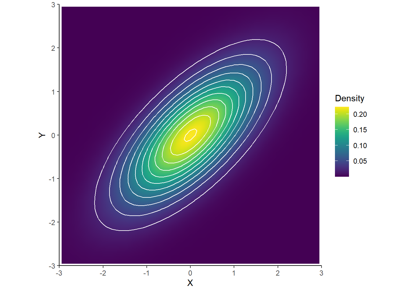
• A Bivariate Normal Density has elliptical contours. For each height \(c>0\) the set \(\{(x,y): f_{X, Y}(x,y)=c\}\) is an ellipse. The density decreases as \((x, y)\) moves away from \((\mu_X, \mu_Y)\), most steeply along the minor axis of the ellipse, and least steeply along the major of the ellipse.
• A scatterplot of \((x,y)\) pairs generated from a Bivariate Normal distribution will have a rough linear association and the cloud of points will resemble an ellipse.
• If \(X\) and \(Y\) have a Bivariate Normal distribution, then the marginal distributions are also Normal: \(X\) has a Normal\(\left(\mu_X,\sigma_X\right)\) distribution and \(Y\) has a Normal\(\left(\mu_Y,\sigma_Y\right)\).
• If \(X\) and \(Y\) have a Bivariate Normal distribution and \(\text{Corr}(X, Y)=0\) then \(X\) and \(Y\) are independent. (Remember, in general it is possible to have situations where the correlation is 0 but the random variables are not independent.)
• \(X\) and \(Y\) have a Bivariate Normal distribution if and only if every linear combination of \(X\) and \(Y\) has a Normal distribution. That is, \(X\) and \(Y\) have a Bivariate Normal distribution if and only if \(aX+bY+c\) has a Normal distribution for all \(a\), \(b\), \(c\).

Figure 15.2: Bivariate Normal distribution with two conditional slices highlighted.

Figure 15.3: Two conditional Normal distributions.

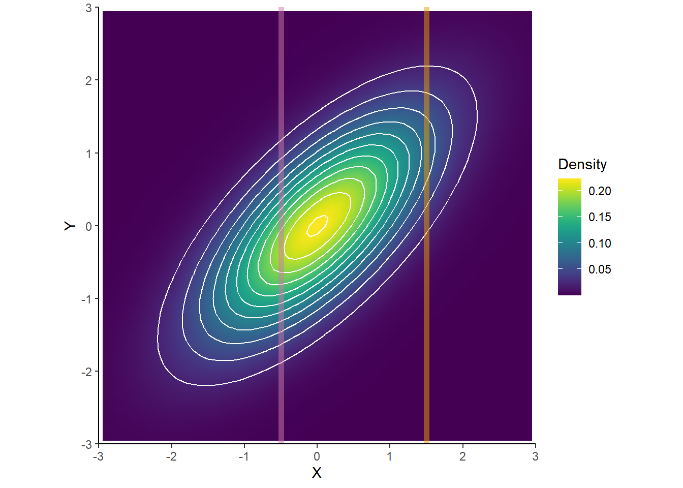
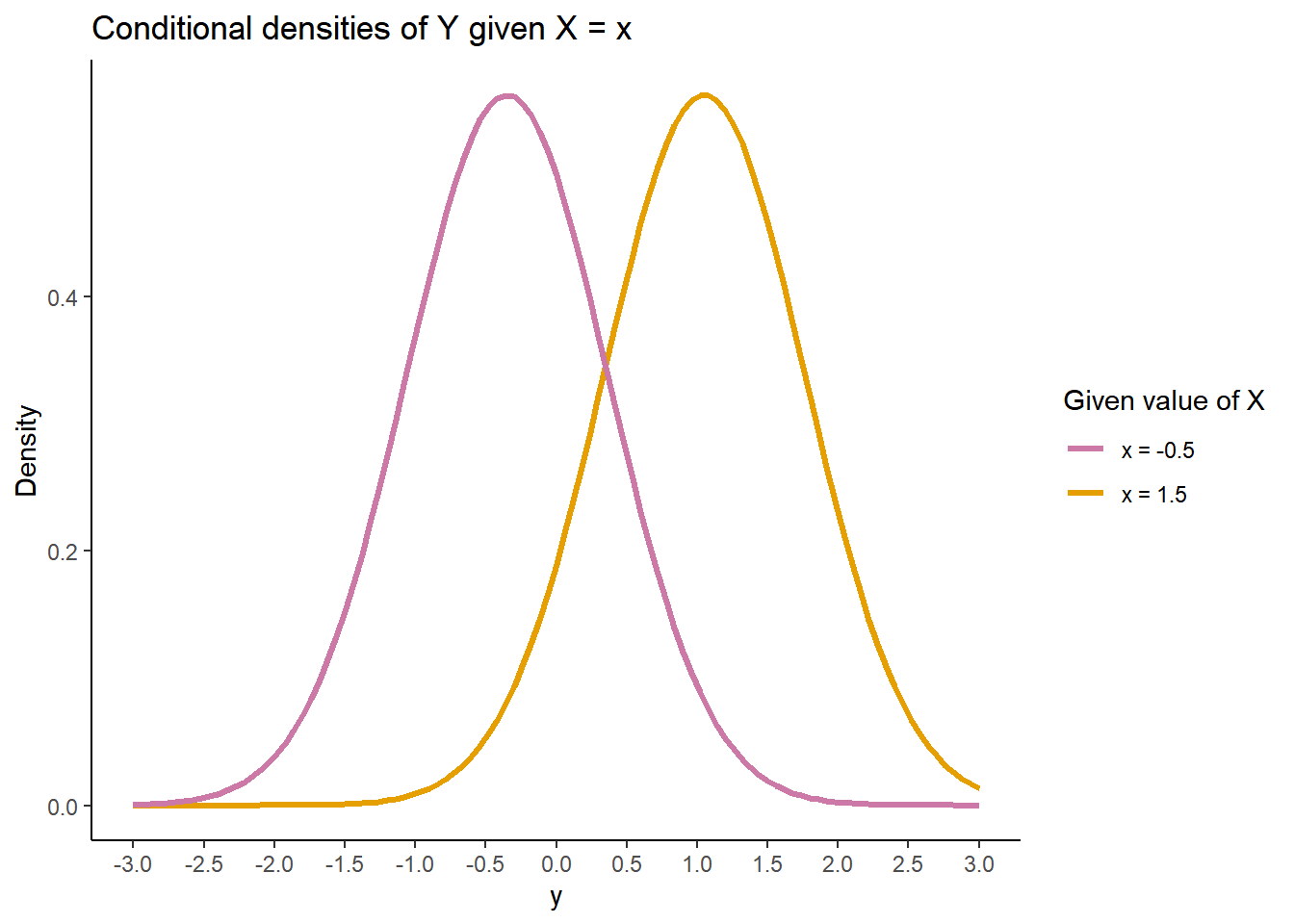
• If \(X\) and \(Y\) have a Bivariate Normal distribution then any conditional distribution is Normal. The conditional distribution of \(Y\) given \(X=x\) is

\[ N\left(\mu_Y + \frac{\rho\sigma_Y}{\sigma_X}\left(x-\mu_X\right),\;\sigma_Y\sqrt{1-\rho^2}\right) \]

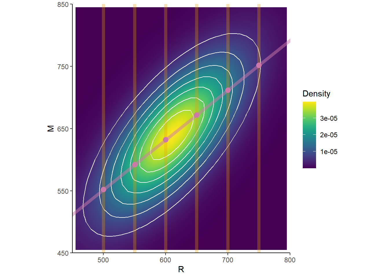
• The conditional expected value of \(Y\) given \(X=x\) is a linear function of \(x\), called the regression line of \(Y\) on \(X\): \[ \text{E}(Y | X=x) = \mu_Y + \rho\sigma_Y\left(\frac{x-\mu_X}{\sigma_X}\right) \]
  • The regression line passes through the point of means \((\mu_X, \mu_Y)\) and has slope \[ \frac{\rho \sigma_Y}{\sigma_X} \]
  • The regression line estimates that if the given \(x\) value is \(z\) SDs above the mean of \(X\), then the corresponding \(Y\) values will be, on average, \(\rho z\) SDs away from the mean of \(Y\) \[ \frac{\text{E}(Y|X=x) - \mu_Y}{\sigma_Y} = \rho\left(\frac{x-\mu_X}{\sigma_X}\right) \]
  • Since \(|\rho|\le 1\), for a given \(x\) value the corresponding \(Y\) values will be, on average, relatively closer to the mean of \(Y\) than the given \(x\) value is to the mean of \(X\). This is known as regression to the mean.
• For Bivariate Normal distributions, the conditional variance of \(Y\) given \(X=x\) does not depend on \(x\): \[ \text{SD}(Y |X = x) = \sigma_Y\sqrt{1-\rho^2} \]

Example 15.1

Suppose that SAT Math (\(M\)) and Reading (\(R\)) scores of CalPoly students have a Bivariate Normal distribution. Math scores have mean 640 and SD 80, Reading scores have mean 610 and SD 70, and the correlation between scores is 0.7.

1. Identify the distribution of Math scores. Find the probability that a student has a Math score above 700.
   
   
   
   
   
2. Compute and interpret \(\text{E}(M|R = 700)\).
   
   
   
   
   
3. Compute and interpret \(\text{SD}(M|R = 700)\).
   
   
   
   
   
4. Identify the conditional distribution of Math scores given the Reading score is 700. Find the probability that a student has a higher Math than Reading score if the student scores 700 on Reading.
   
   
   
   
   
5. Compute and interpret \(\text{E}(M|R = 550)\).
   
   
   
   
   
6. Compute and interpret \(\text{SD}(M|R = 550)\).
   
   
   
   
   
7. Identify the conditional distribution of Math scores given the Reading score is 550. Find the probability that a student has a higher Math than Reading score if the student scores 550 on Reading.
   
   
   
   
   
8. Describe how you could simulate a single \((M, R)\) pair.
   
   
   
   
   
9. Find and interpret \(\text{E}(M|R)\).
   
   
   
   
   

Figure 15.4: A Bivariate Normal distribution with some conditional distributions and conditional expected values highlighted.

N_rep = 10000

R = rnorm(N_rep, 610, 70)
M = rnorm(N_rep, 640 + 0.7 * 80 * (R - 610) / 70, 80 * sqrt(1 - 0.7 ^ 2))

plot(R, M)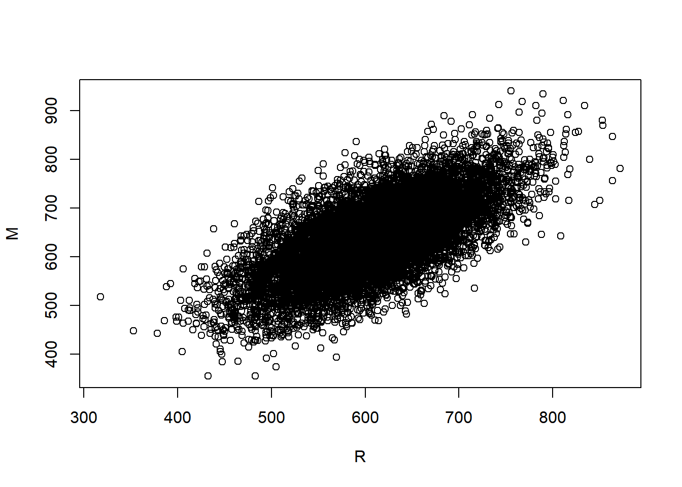

ggplot(data.frame(R, M), aes(x = R, y = M)) +
  stat_density_2d(aes(fill = ..level..), geom = "polygon", colour="white")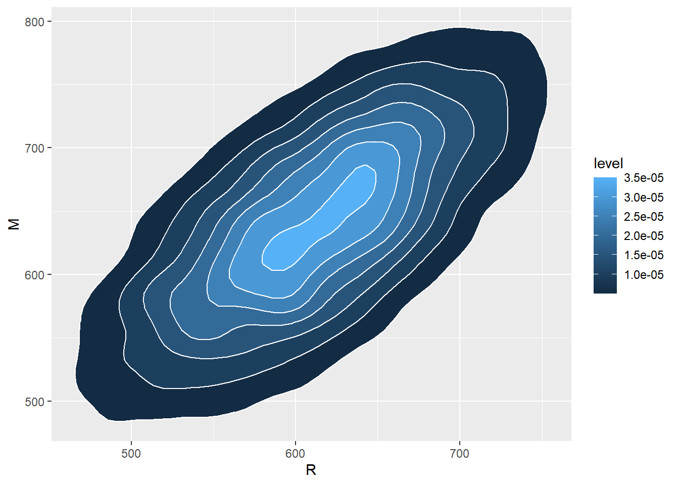

cor(R, M)

[1] 0.6867692

mean(R)

[1] 609.8806

sd(R)

[1] 69.73702

mean(M)

[1] 639.406

sd(M)

[1] 78.31964

• If the pair \((X,Y)\) has a joint Normal distribution then each of \(X\) and \(Y\) has a Normal distribution.
• But the converse is not true. That is, if each of \(X\) and \(Y\) has a Normal distribution, it is not necessarily true that the pair \((X, Y)\) has a joint Normal distribution
• However, if \(X\) and \(Y\) are independent and each of \(X\) and \(Y\) has a Normal distribution, then the pair \((X, Y)\) has a joint Normal distribution. (But joint Normal is much more general that two independent Normal random variables.)