7 Variance Explained and Modeling (9/18)
Our plan for today:
Review the concept of variance as it relates to correlational statistics;
apply knowledge from music education literature to develop hypotheses that explain variance;
and draw conceptual models of our hypotheses.
While we critically examine the research questions for our class projects;
and identify the statistical procedures and potential outcomes of each research question.

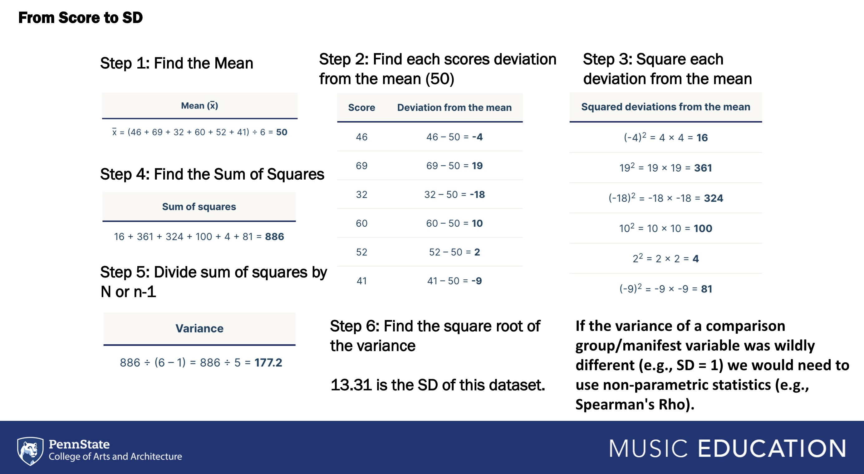
Variance is a measure of variability. To calculate variance, square the standard deviation. SDs are themselves derived from variance and reflect variance in terms of the measured scale—as they are the square root of the sum of squares. They are typically smaller and easier to understand. So far, we have considered variance through statistical assumptions for tests like Pearson’s R (i.e., homogeneity of variance) and assessments of the normality of a distribution (i.e., kurtosis).
For example, on a test where possible scores fall between 0 and 100.
Where M = 70, SD = 0, Variance = 0: Everyone received the same score, 100% of scores are 70.
Where M = 70, SD = 2, Variance = 4: A large majority of participants received the same score and it was clustered around the mean, 95% of scores between 66-74).
Where M = 70, SD = 8, Variance = 64: There is a moderate to large amount of variance across scores, 95% of scores between 54 and 86.
Much of our work as quantitative researchers is to completely and succinctly explain variance. Practically, explained variance refers to the proportion of which a statistical model accounts (e.g., a correlation test counts) for the dispersion in a dataset.
7.1 R-Squared
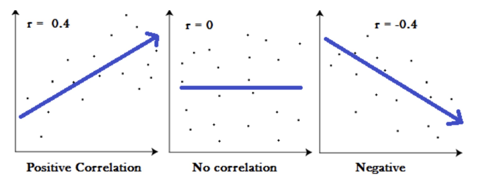
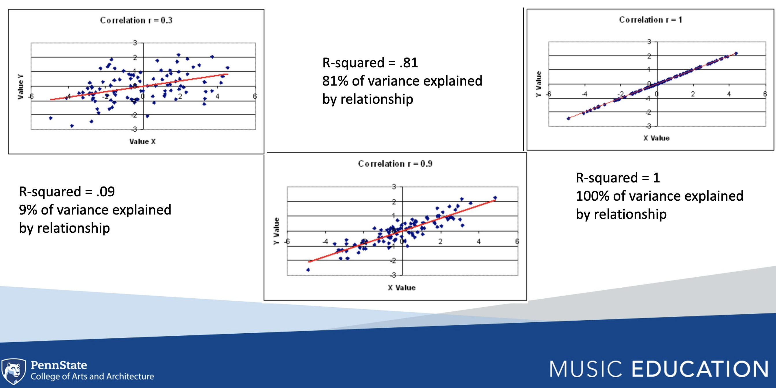
R-squared is a common metric used to assess and interpret variance explained in a correlational model. Square r to calculate r-squared. The outcome can be stated as a percentage of the variance explained by the relationship. For example, the first pane below has an r of .4, and an r-squared value of .16, thus indicating that 16% of the relationship in the y-axis is explained by the variable in the x-axis. What about the third pane?
7.1.1 Model Drawing Demo
We create and test theoretical models to explain variance effectively. It might start with a hunch, or following the review of literature related to your problem or research interest area.
7.1.1.1 Correlation
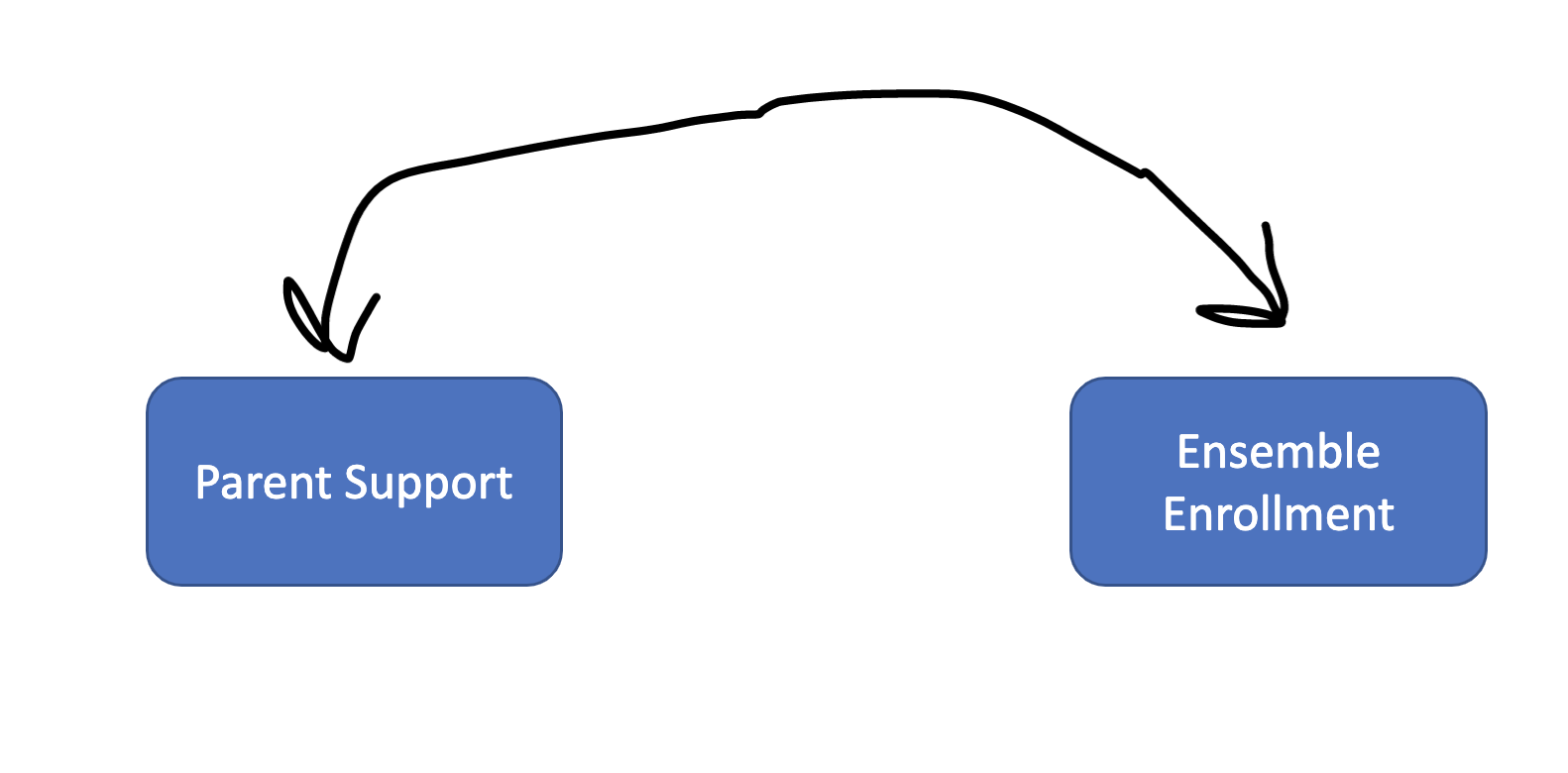
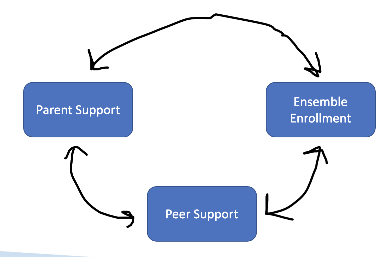
Two variables can be correlated and display a pattern of covariance. Below is a drawing of a correlational model that would explain covariance* in ensemble enrollment and parent support.
RQ: What is the relationship between ensemble enrollment and parent support?
Two or more variables can be correlated in (e.g., parent support and peer support can be correlated, which are each correlated with ensemble enrollment). This type of model would explain covariance in ensemble enrollment and parent support, covariance in ensemble enrollment and peer support, and covariance in peer support and parent support
RQ1: What is the relationship between ensemble enrollment and parent support?
RQ2: What is the relationship between ensemble enrollment and peer support?
RQ3: What is the relationship between peer support and parent support?
Variance in ensemble enrollment is explained one variable at a time.
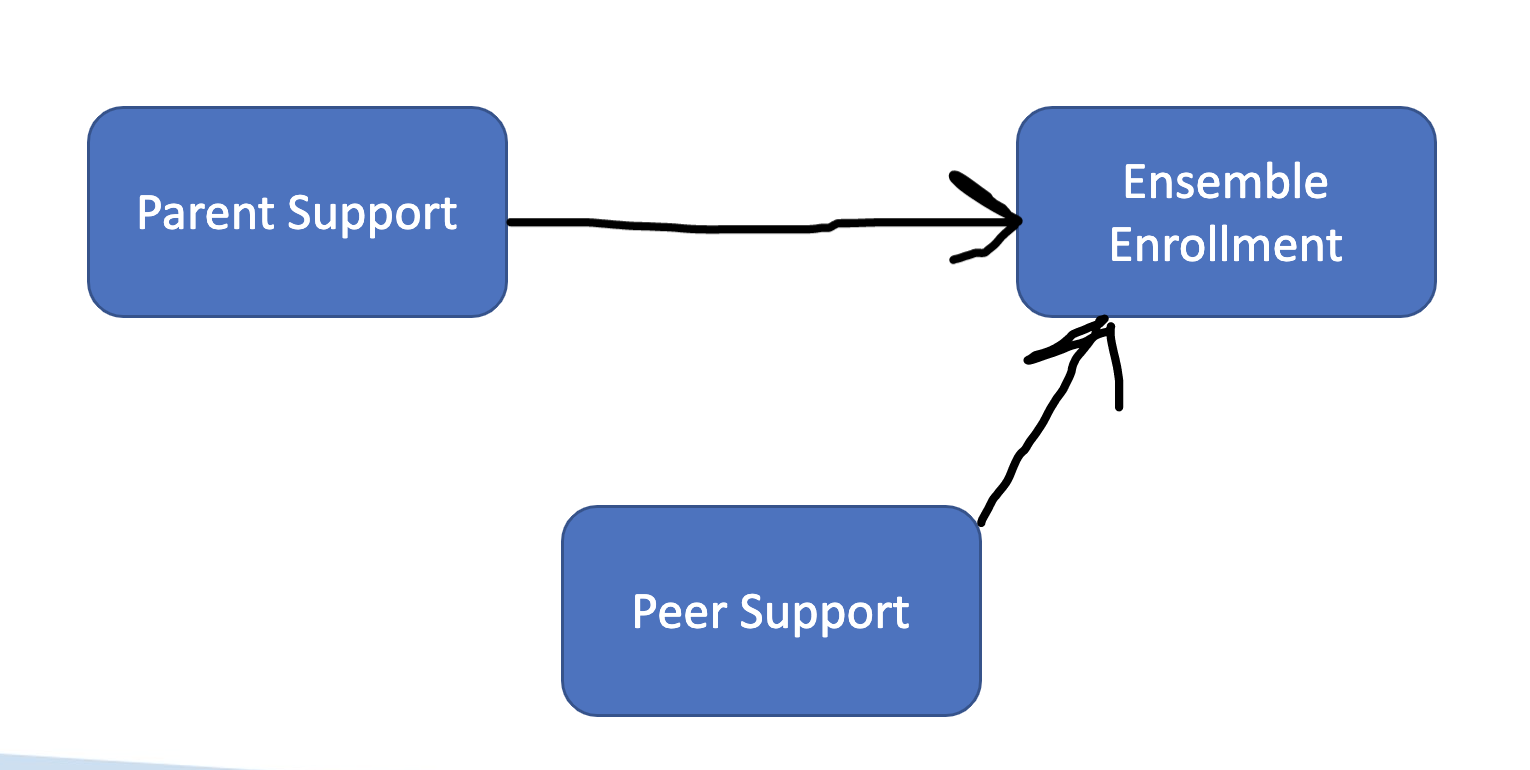
7.1.1.2 Regression
We use regression to explain variance in a single variable as the result of multiple predictors. In regression, we use values of one or more variables to predict values in another. As such, ensemble enrollment can be conceived of as a function of peer and parent support—where we can ascertain the extent to which changes in parent/peer support predict changes in ensemble enrollment.
Researchers can use regression coefficients to infer beyond the direction and magnitude of relationships and discuss changes in Y due to specific changes in X (e.g., for every increase of 1 unit in Y, X increases .5).
The unstandardized regression formula is Y = a + bX where a is the intercept (where the line of best fit crosses the y-axis) and b is the slope of the regression line (½ is up 1 over 2). Put otherwise, a is the value of Y when X = 0 and b is the regression coefficient. The null hypothesis of the regression model is that independent variables are not able to significantly predict the dependent variable (i.e., the slope or standardized beta weight is 0, and that the predictor variable had no impact on the dependent variable).
We also calculate R-squared to explain variance in this model, but the value is referring to total variance explained by the effect of a combination of variables on an outcome variables (e.g., parent support explains 20% of variance in ensemble enrollment while peer support explains 15% of variance. R-squared would be .35 in this example).
RQ1: To what extent does parent support predict ensemble enrollment?
RQ2: To what extent does peer support predict ensemble enrollment?
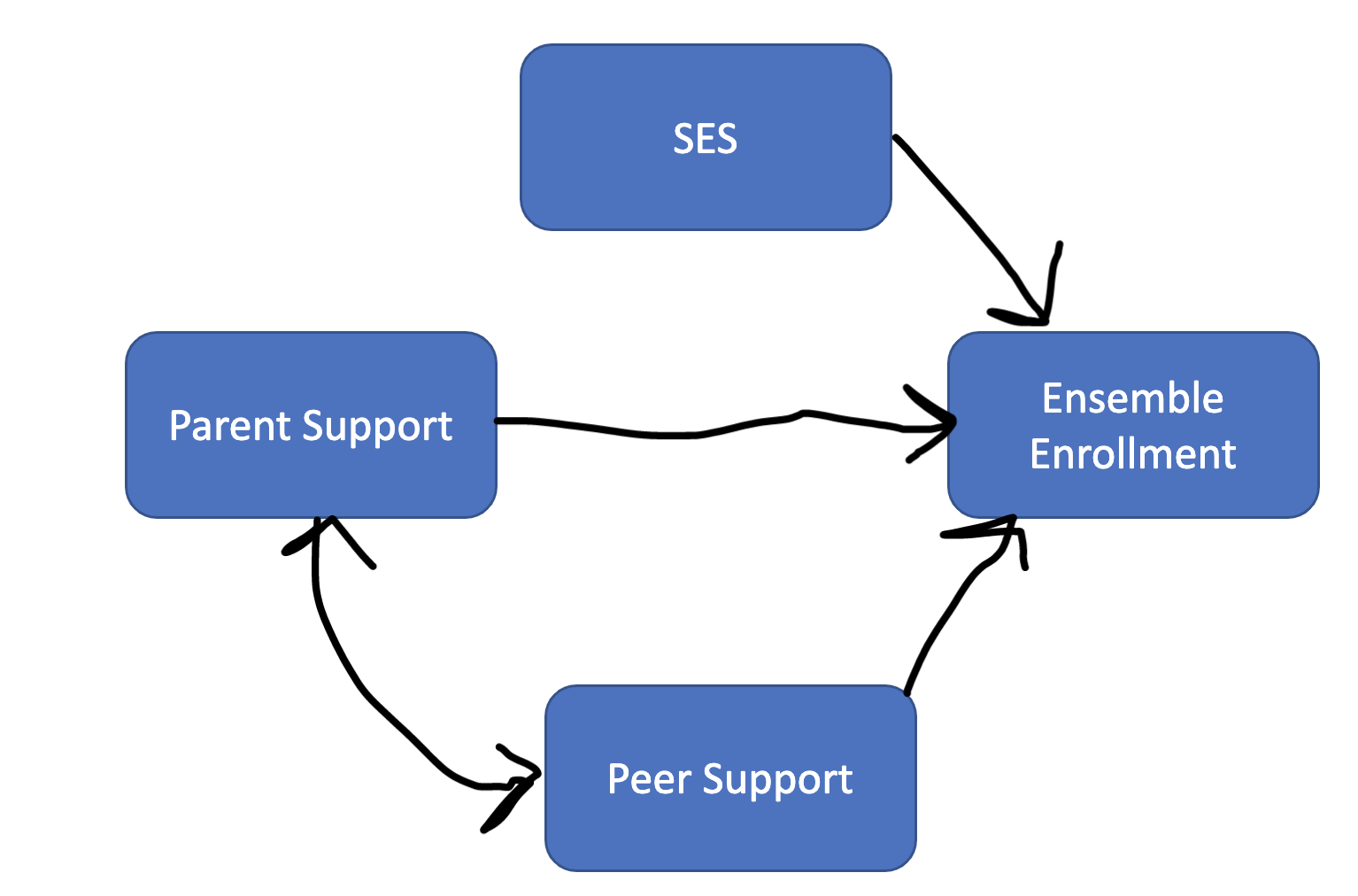
We can estimate regression equations (effect of X on Y) alongside correlations (relationship between X and Y)
RQ1: What is the relationship between parent and peer support?
RQ2: What is the effect of SES on ensemble enrollment?
RQ3: What is the effect of peer support on ensemble enrollment?
RQ4: What is the effect of parent support on ensemble enrollment?
RQ5: What are the best set of predictors for ensemble enrollment? (what group of variables creates the highest r-squared value)
Let’s practice explaining variance using the participation data set revisiting RQ5
What are the best set of predictors for ensemble enrollment?
#install.packages('olsrr')
library(olsrr)
##
## Attaching package: 'olsrr'## The following object is masked from 'package:datasets':
##
## riverslibrary(tidyverse)
library(rstatix)
data <- read_csv('participationdatashort.csv')## Rows: 42 Columns: 9## ── Column specification ────────────────────────────────────────────────────────
## Delimiter: ","
## chr (3): GradeLevel, Class, Gender
## dbl (6): intentionscomp, needscomp, valuescomp, parentsupportcomp, peersuppo...
##
## ℹ Use `spec()` to retrieve the full column specification for this data.
## ℹ Specify the column types or set `show_col_types = FALSE` to quiet this message.data## # A tibble: 42 × 9
## intentionscomp needscomp value…¹ paren…² peers…³ SESComp Grade…⁴ Class Gender
## <dbl> <dbl> <dbl> <dbl> <dbl> <dbl> <chr> <chr> <chr>
## 1 8 58 55 5 9 2 eighth… band Male
## 2 18 54 79 10 10 2.4 sevent… orch… Female
## 3 6 61 53 6 5 3 sevent… band Female
## 4 15 55 72 11 6 3 sevent… orch… Female
## 5 16 47 59 10 8 2.6 sevent… band Male
## 6 17 58 76 13 13 3 sevent… band Male
## 7 18 54 68 11 8 3 sevent… band Female
## 8 6 37 43 6 5 2.4 sevent… band Female
## 9 16 33 44 5 7 3 sevent… orch… Male
## 10 3 42 42 6 7 2.4 eighth… band Female
## # … with 32 more rows, and abbreviated variable names ¹valuescomp,
## # ²parentsupportcomp, ³peersupportcomp, ⁴GradeLevelAssess correlations for the target variable, intentionscomp.
data %>% cor_test(intentionscomp, method = "pearson")## # A tibble: 5 × 8
## var1 var2 cor statis…¹ p conf.…² conf.…³ method
## <chr> <chr> <dbl> <dbl> <dbl> <dbl> <dbl> <chr>
## 1 intentionscomp needscomp 0.12 0.731 4.69e-1 -0.198 0.409 Pears…
## 2 intentionscomp valuescomp 0.54 4.00 2.82e-4 0.280 0.732 Pears…
## 3 intentionscomp parentsupportcomp 0.44 3.08 3.69e-3 0.155 0.655 Pears…
## 4 intentionscomp peersupportcomp 0.36 2.42 2 e-2 0.0604 0.597 Pears…
## 5 intentionscomp SESComp 0.19 1.20 2.39e-1 -0.129 0.474 Pears…
## # … with abbreviated variable names ¹statistic, ²conf.low, ³conf.high#only strongest correlate
mod1 <- lm(intentionscomp ~ valuescomp, data = data)
summary(mod1)##
## Call:
## lm(formula = intentionscomp ~ valuescomp, data = data)
##
## Residuals:
## Min 1Q Median 3Q Max
## -8.0495 -2.5906 0.3278 3.3858 9.0502
##
## Coefficients:
## Estimate Std. Error t value Pr(>|t|)
## (Intercept) -2.24961 3.81040 -0.590 0.558427
## valuescomp 0.23181 0.05794 4.001 0.000282 ***
## ---
## Signif. codes: 0 '***' 0.001 '**' 0.01 '*' 0.05 '.' 0.1 ' ' 1
##
## Residual standard error: 4.521 on 38 degrees of freedom
## (2 observations deleted due to missingness)
## Multiple R-squared: 0.2964, Adjusted R-squared: 0.2779
## F-statistic: 16.01 on 1 and 38 DF, p-value: 0.0002816#all significant correlates
mod2 <- lm(intentionscomp ~ valuescomp + parentsupportcomp + peersupportcomp, data = data)
summary(mod2)##
## Call:
## lm(formula = intentionscomp ~ valuescomp + parentsupportcomp +
## peersupportcomp, data = data)
##
## Residuals:
## Min 1Q Median 3Q Max
## -7.8776 -2.9300 -0.1856 2.8321 9.5002
##
## Coefficients:
## Estimate Std. Error t value Pr(>|t|)
## (Intercept) -3.71794 3.81496 -0.975 0.3363
## valuescomp 0.16459 0.06811 2.417 0.0209 *
## parentsupportcomp 0.36952 0.28790 1.284 0.2075
## peersupportcomp 0.33983 0.27133 1.252 0.2185
## ---
## Signif. codes: 0 '***' 0.001 '**' 0.01 '*' 0.05 '.' 0.1 ' ' 1
##
## Residual standard error: 4.431 on 36 degrees of freedom
## (2 observations deleted due to missingness)
## Multiple R-squared: 0.3598, Adjusted R-squared: 0.3064
## F-statistic: 6.744 on 3 and 36 DF, p-value: 0.0009997#all significant and non-significant correlates
mod3 <- lm(intentionscomp ~ needscomp + valuescomp + SESComp, data = data)
summary(mod3)##
## Call:
## lm(formula = intentionscomp ~ needscomp + valuescomp + SESComp,
## data = data)
##
## Residuals:
## Min 1Q Median 3Q Max
## -9.4908 -2.3724 -0.0537 2.7269 7.3723
##
## Coefficients:
## Estimate Std. Error t value Pr(>|t|)
## (Intercept) -4.14483 6.64590 -0.624 0.5371
## needscomp -0.24879 0.12096 -2.057 0.0477 *
## valuescomp 0.33711 0.06914 4.876 2.66e-05 ***
## SESComp 3.30969 1.72158 1.922 0.0632 .
## ---
## Signif. codes: 0 '***' 0.001 '**' 0.01 '*' 0.05 '.' 0.1 ' ' 1
##
## Residual standard error: 4.094 on 33 degrees of freedom
## (5 observations deleted due to missingness)
## Multiple R-squared: 0.4408, Adjusted R-squared: 0.39
## F-statistic: 8.671 on 3 and 33 DF, p-value: 0.0002202We can also use the olsrr library to run stepwise regression and identify the best fitting model. Insert a period instead of variables to call all variables in the dataset.
model <- lm(intentionscomp ~ ., data = data)
modelchoice <- ols_step_all_possible(model) %>% arrange(desc(adjr)) %>% filter(n <= 4)
View(head(modelchoice))
7.1.2 Practice Activity
Considering your developing research project, take notes using the following steps:
Step 1: Refer to your research questions for your class project—list out all variables that are involved in your RQs.
Step 2: Question by question, draw a theoretical model using curvilinear lines for correlation and straight lines for regression.
Step 3: Draw a model that includes all your research questions simultaneously. For descriptive research questions, you might just place an * on the variable and make a note that you will describe the variable in question.
Step 4: Reconsider your research questions. Are they interesting/useful? Do they address the problem you’ve identified? Can they be worded in a better way? Should you change them or add something new?
Step 5: Redraw your model.
Step 6: Label your final model with your RQs.