6 Correlational Statistics (9/12-9/14)
Onto correlation! Although we will still consistently reference descriptive statistics, and issues of measurement (e.g., validity, reliability, generalizability), we now move into the correlational realm. This week, we will:
- Discuss correlational concepts, including significance (practical and statistical), magnitude, and direction.
- Distinguish between four correlational approaches to data analysis, and know when to use them.
- Interact with the statistical assumptions of correlation, specifically for Pearson’s R.
- Evaluate research scenarios for the appropriate analysis approach.
- Practice correlational analysis as a group and individually in both SPSS and R.
Due Wednesday: Read russell chapter 16 on Cronbach’s alpha/reliability
6.1 Correlational Concepts
Moreover, correlation captures how two or more variables move together to express the relationship between variables. Correlations can be attenuated (i.e., weakened) by other factors, including the reliability of measured variables, range restrictions (e.g., ceiling or floor effects) and low sample size (>30 participants typically desired).
A “correlational” investigation implies the desire to find a pattern or relationship between variable (e.g., what is the relationship between x and y);
Correlational analysis is commonly employed in survey studies as an additional step beyond basic descriptive statistics;
Correlational research designs can be used as a precursor to an experiment (e.g., determining what variables are correlated with student effort before trying to conduct an experiment designed to improve student effort among adolescents).
Even if your final goal is regression or an inferential statistical test, correlations are useful to look at during exploratory data analysis before trying to fit a predictive model.
6.1.1 Four Components of Correlational Analysis
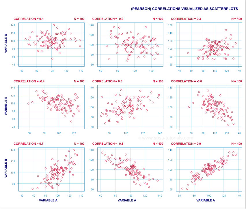
Correlation coefficients, or the statistics that emerge from conducting correlational analyses, are returned as a number between -1 and 1. The number itself tells us about the strength of the relationship (i.e., [0-.29] is weak, [.3-.69] is moderate, and [.7-1] is strong);
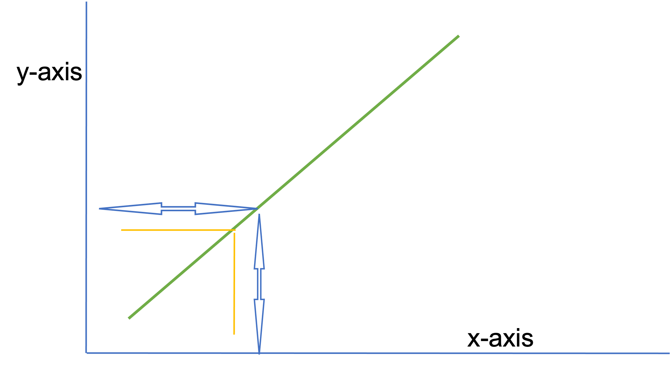
The valence of the relationship (i.e., positive/negative, direct/indirect) indicates the quality of the relationship (e.g., as age increases so does knowledge is a direct relationship, as the temperature goes down the amount of students wearing coats increases is an indirect relationship).
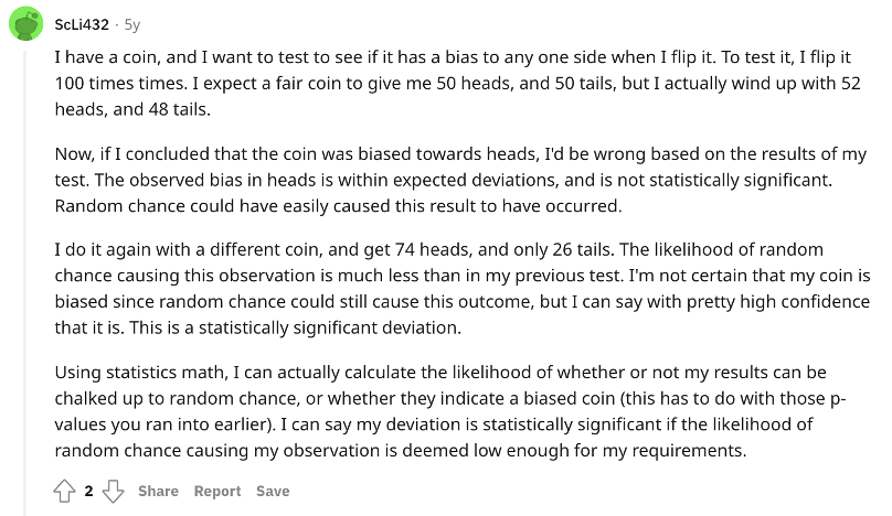
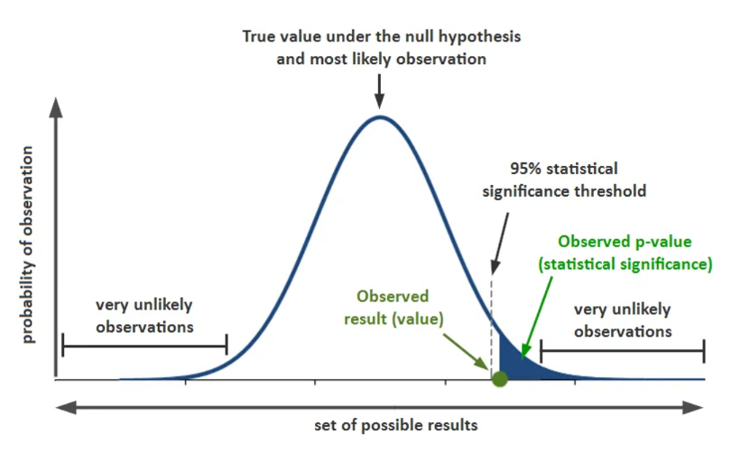
We then use statistical significance (p-values) to indicate whether our findings are due to chance or likely not due to chance. For example, if you set your apriori alpha level to .05 for a correlation test that measures alignment of math and music performance scores and find a strong direct and significant correlation (r = .71, p = .03) there is only a 3% probability that the evidence for the correlation is larger than can reasonably be explained as a chance occurrence.
Practical significance is also considered. For instance, if you have a significant, direct, but weak correlation (e.g., r = .09, p = .049) there may be no practical significance to the connection whereas findings from a stronger association (e.g., r = .40, p = .049) may be extrapolated or scrutinized further.
6.1.2 Considering Correlation Approaches and Data Types
Although the Pearson Correlation Coeffecient is the most popular method, the correlational approach you use depends on the type of data you have. See the table below for a breakdown of each correlational test and when to use it.
| Test | R Function | When to use it | Visualized |
|---|---|---|---|
| Chi-Square | chisq.test() |
|
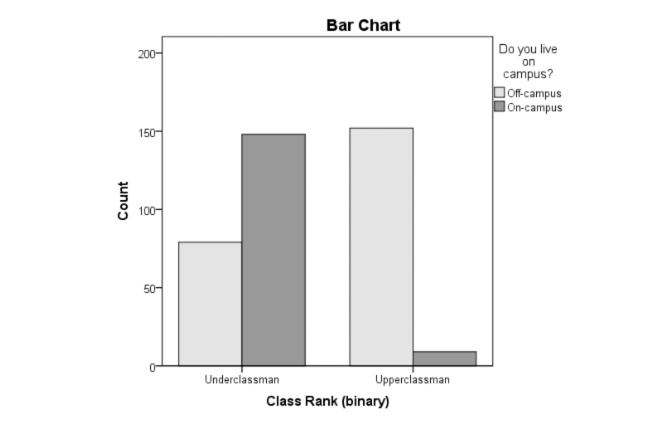 |
| Spearman’s Rho | cor.test(method = "spearman") |
|
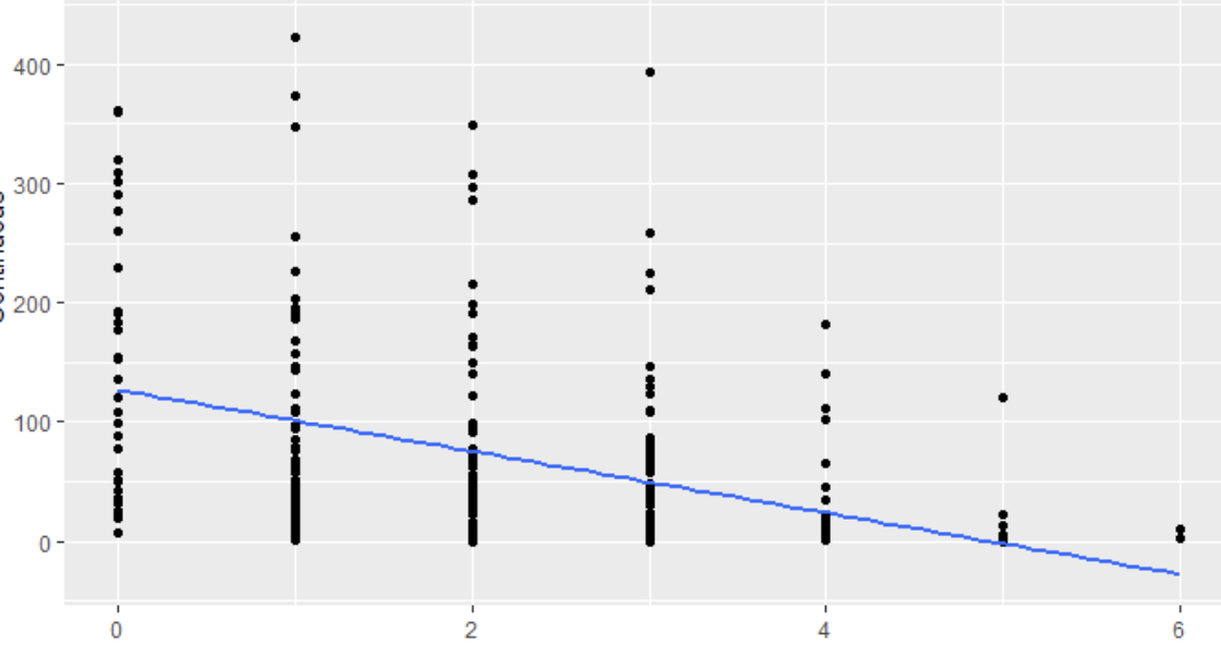 |
| Pearson’s R | cor.test(method = "pearson") |
|
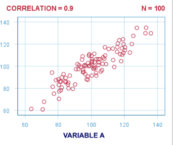 |
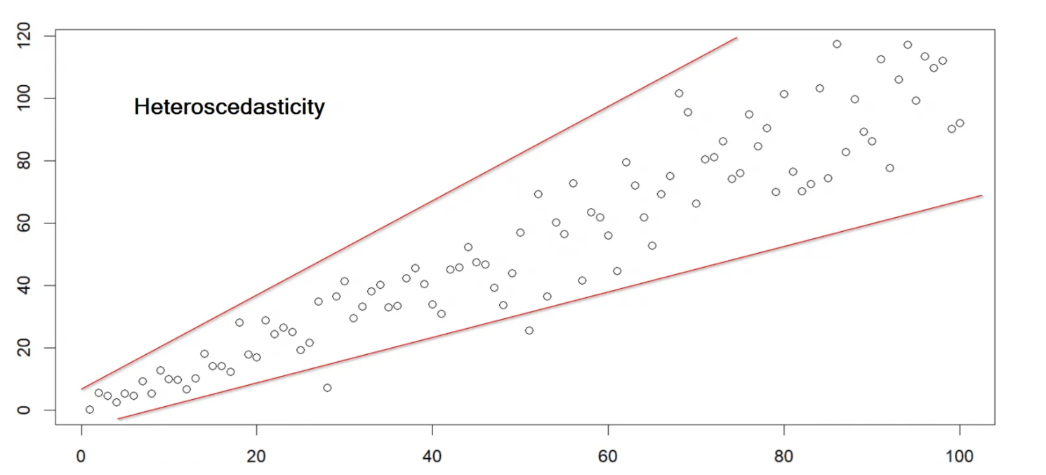
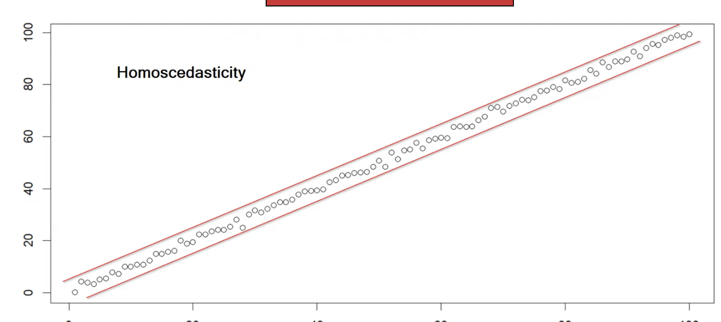
Homoscedasticity means “same variance,” in that data points vary at a similar rate across the spectrum of scores. Heteroscedasticity means “different variance.”
6.2 Correlation Participation Case Study
We will be using a built-in dataset from the participationdatashort.csv file that contains information on elective intentions for ensemble participation.
Install a new package using this chunk.
install.packages('DataExplorer')
install.packages('report')
install.packages('readxl')
install.packages('rstatix')
Load libraries using this chunk.
library(tidyverse)
library(DataExplorer)
library(psych)
library(report)
library(readxl)
library(rstatix)
##
## Attaching package: 'rstatix'## The following object is masked from 'package:stats':
##
## filterTo get a quick look at many facets of a dataset in one line of code, try DataExplorer. DataExplorer includes an automated data exploration process for analytic tasks and predictive modeling. Simply run the function create_report() on a data frame to produce multiple plots and tables related to descriptive and correlation related analyses. Use the summary(), str(), and psych::describe() functions to examine and assess the variables in the dataset for normality.
data <- read_csv('participationdatashort.csv')## Rows: 42 Columns: 9
## ── Column specification ────────────────────────────────────────────────────────
## Delimiter: ","
## chr (3): GradeLevel, Class, Gender
## dbl (6): intentionscomp, needscomp, valuescomp, parentsupportcomp, peersuppo...
##
## ℹ Use `spec()` to retrieve the full column specification for this data.
## ℹ Specify the column types or set `show_col_types = FALSE` to quiet this message.DataExplorer::create_report(data)##
##
## processing file: report.rmd##
|
| | 0%
|
|.. | 2%
## inline R code fragments
##
##
|
|... | 5%
## label: global_options (with options)
## List of 1
## $ include: logi FALSE
##
##
|
|..... | 7%
## ordinary text without R code
##
##
|
|....... | 10%
## label: introduce
##
|
|........ | 12%
## ordinary text without R code
##
##
|
|.......... | 14%
## label: plot_intro##
|
|............ | 17%
## ordinary text without R code
##
##
|
|............. | 19%
## label: data_structure
##
|
|............... | 21%
## ordinary text without R code
##
##
|
|................. | 24%
## label: missing_profile##
|
|.................. | 26%
## ordinary text without R code
##
##
|
|.................... | 29%
## label: univariate_distribution_header
##
|
|...................... | 31%
## ordinary text without R code
##
##
|
|....................... | 33%
## label: plot_histogram##
|
|......................... | 36%
## ordinary text without R code
##
##
|
|........................... | 38%
## label: plot_density
##
|
|............................ | 40%
## ordinary text without R code
##
##
|
|.............................. | 43%
## label: plot_frequency_bar##
|
|................................ | 45%
## ordinary text without R code
##
##
|
|................................. | 48%
## label: plot_response_bar
##
|
|................................... | 50%
## ordinary text without R code
##
##
|
|..................................... | 52%
## label: plot_with_bar
##
|
|...................................... | 55%
## ordinary text without R code
##
##
|
|........................................ | 57%
## label: plot_normal_qq##
|
|.......................................... | 60%
## ordinary text without R code
##
##
|
|........................................... | 62%
## label: plot_response_qq
##
|
|............................................. | 64%
## ordinary text without R code
##
##
|
|............................................... | 67%
## label: plot_by_qq
##
|
|................................................ | 69%
## ordinary text without R code
##
##
|
|.................................................. | 71%
## label: correlation_analysis##
|
|.................................................... | 74%
## ordinary text without R code
##
##
|
|..................................................... | 76%
## label: principal_component_analysis##
|
|....................................................... | 79%
## ordinary text without R code
##
##
|
|......................................................... | 81%
## label: bivariate_distribution_header
##
|
|.......................................................... | 83%
## ordinary text without R code
##
##
|
|............................................................ | 86%
## label: plot_response_boxplot
##
|
|.............................................................. | 88%
## ordinary text without R code
##
##
|
|............................................................... | 90%
## label: plot_by_boxplot
##
|
|................................................................. | 93%
## ordinary text without R code
##
##
|
|................................................................... | 95%
## label: plot_response_scatterplot
##
|
|.................................................................... | 98%
## ordinary text without R code
##
##
|
|......................................................................| 100%
## label: plot_by_scatterplot## output file: /Users/jbh6331/Desktop/R/540/report.knit.md## /Applications/RStudio.app/Contents/MacOS/quarto/bin/pandoc +RTS -K512m -RTS /Users/jbh6331/Desktop/R/540/report.knit.md --to html4 --from markdown+autolink_bare_uris+tex_math_single_backslash --output /Users/jbh6331/Desktop/R/540/report.html --lua-filter /Users/jbh6331/Library/R/x86_64/4.2/library/rmarkdown/rmarkdown/lua/pagebreak.lua --lua-filter /Users/jbh6331/Library/R/x86_64/4.2/library/rmarkdown/rmarkdown/lua/latex-div.lua --self-contained --variable bs3=TRUE --standalone --section-divs --table-of-contents --toc-depth 6 --template /Users/jbh6331/Library/R/x86_64/4.2/library/rmarkdown/rmd/h/default.html --no-highlight --variable highlightjs=1 --variable theme=yeti --mathjax --variable 'mathjax-url=https://mathjax.rstudio.com/latest/MathJax.js?config=TeX-AMS-MML_HTMLorMML' --include-in-header /var/folders/_t/4fctbs650sqbl5b86n88pnbdb8jsl9/T//RtmpUInMZ0/rmarkdown-str183db5c560c1d.html##
## Output created: report.html#summary(data)
#str(data)
#psych::describe(data)subsetdata <- data %>% select(intentionscomp, needscomp, valuescomp, parentsupportcomp, peersupportcomp, SESComp)6.2.1 Assessing Correlation with BaseR, psych, Rstatix, and Report
cor.test(subsetdata$needscomp, subsetdata$valuescomp)##
## Pearson's product-moment correlation
##
## data: subsetdata$needscomp and subsetdata$valuescomp
## t = 4.3612, df = 37, p-value = 9.938e-05
## alternative hypothesis: true correlation is not equal to 0
## 95 percent confidence interval:
## 0.3273518 0.7587153
## sample estimates:
## cor
## 0.5826861# Correlation test between two variables
subsetdata %>% cor_test(needscomp, valuescomp, method = "pearson")## # A tibble: 1 × 8
## var1 var2 cor statistic p conf.low conf.high method
## <chr> <chr> <dbl> <dbl> <dbl> <dbl> <dbl> <chr>
## 1 needscomp valuescomp 0.58 4.36 0.0000994 0.327 0.759 Pearson# Correlation of one variable against all
subsetdata %>% cor_test(intentionscomp, method = "pearson")## # A tibble: 5 × 8
## var1 var2 cor statis…¹ p conf.…² conf.…³ method
## <chr> <chr> <dbl> <dbl> <dbl> <dbl> <dbl> <chr>
## 1 intentionscomp needscomp 0.12 0.731 4.69e-1 -0.198 0.409 Pears…
## 2 intentionscomp valuescomp 0.54 4.00 2.82e-4 0.280 0.732 Pears…
## 3 intentionscomp parentsupportcomp 0.44 3.08 3.69e-3 0.155 0.655 Pears…
## 4 intentionscomp peersupportcomp 0.36 2.42 2 e-2 0.0604 0.597 Pears…
## 5 intentionscomp SESComp 0.19 1.20 2.39e-1 -0.129 0.474 Pears…
## # … with abbreviated variable names ¹statistic, ²conf.low, ³conf.high# Pairwise correlation test between all variables
subsetdata %>% cor_test(method = "pearson")## # A tibble: 36 × 8
## var1 var2 cor stati…¹ p conf.…² conf.…³ method
## <chr> <chr> <dbl> <dbl> <dbl> <dbl> <dbl> <chr>
## 1 intentionscomp intentionscomp 1 Inf 0 1 1 Pears…
## 2 intentionscomp needscomp 0.12 0.731 4.69e-1 -0.198 0.409 Pears…
## 3 intentionscomp valuescomp 0.54 4.00 2.82e-4 0.280 0.732 Pears…
## 4 intentionscomp parentsupportcomp 0.44 3.08 3.69e-3 0.155 0.655 Pears…
## 5 intentionscomp peersupportcomp 0.36 2.42 2 e-2 0.0604 0.597 Pears…
## 6 intentionscomp SESComp 0.19 1.20 2.39e-1 -0.129 0.474 Pears…
## 7 needscomp intentionscomp 0.12 0.731 4.69e-1 -0.198 0.409 Pears…
## 8 needscomp needscomp 1 Inf 0 1 1 Pears…
## 9 needscomp valuescomp 0.58 4.36 9.94e-5 0.327 0.759 Pears…
## 10 needscomp parentsupportcomp 0.45 3.12 3.43e-3 0.161 0.663 Pears…
## # … with 26 more rows, and abbreviated variable names ¹statistic, ²conf.low,
## # ³conf.high# Compute correlation matrix
cor.mat <- subsetdata %>% cor_mat()
cor.mat## # A tibble: 6 × 7
## rowname intentionscomp needscomp valuescomp parent…¹ peers…² SESComp
## * <chr> <dbl> <dbl> <dbl> <dbl> <dbl> <dbl>
## 1 intentionscomp 1 0.12 0.54 0.44 0.36 0.19
## 2 needscomp 0.12 1 0.58 0.45 -0.0019 0.011
## 3 valuescomp 0.54 0.58 1 0.52 0.3 -0.12
## 4 parentsupportcomp 0.44 0.45 0.52 1 0.25 -0.14
## 5 peersupportcomp 0.36 -0.0019 0.3 0.25 1 -0.1
## 6 SESComp 0.19 0.011 -0.12 -0.14 -0.1 1
## # … with abbreviated variable names ¹parentsupportcomp, ²peersupportcomp# Show the significance levels
cor.mat %>% cor_get_pval()## # A tibble: 6 × 7
## rowname intentionscomp needscomp valuesc…¹ paren…² peersup…³ SESComp
## <chr> <dbl> <dbl> <dbl> <dbl> <dbl> <dbl>
## 1 intentionscomp 0 0.469 0.000282 3.69e-3 2 e- 2 0.239
## 2 needscomp 0.469 0 0.0000994 3.43e-3 9.91e- 1 0.945
## 3 valuescomp 0.000282 0.0000994 0 5.62e-4 5.99e- 2 0.462
## 4 parentsupportcomp 0.00369 0.00343 0.000562 0 1.07e- 1 0.378
## 5 peersupportcomp 0.02 0.991 0.0599 1.07e-1 1.06e-314 0.535
## 6 SESComp 0.239 0.945 0.462 3.78e-1 5.35e- 1 0
## # … with abbreviated variable names ¹valuescomp, ²parentsupportcomp,
## # ³peersupportcomp# Replacing correlation coefficients by symbols
cor.mat %>%
cor_as_symbols() %>%
pull_lower_triangle()## rowname intentionscomp needscomp valuescomp parentsupportcomp
## 1 intentionscomp
## 2 needscomp
## 3 valuescomp + +
## 4 parentsupportcomp . . +
## 5 peersupportcomp . .
## 6 SESComp
## peersupportcomp SESComp
## 1
## 2
## 3
## 4
## 5
## 6# Mark significant correlations
cor.mat %>%
cor_mark_significant()## rowname intentionscomp needscomp valuescomp parentsupportcomp
## 1 intentionscomp
## 2 needscomp 0.12
## 3 valuescomp 0.54*** 0.58****
## 4 parentsupportcomp 0.44** 0.45** 0.52***
## 5 peersupportcomp 0.36* -0.0019 0.3 0.25
## 6 SESComp 0.19 0.011 -0.12 -0.14
## peersupportcomp SESComp
## 1
## 2
## 3
## 4
## 5
## 6 -0.1# Draw correlogram using R base plot
cor.mat %>%
cor_reorder() %>%
pull_lower_triangle() %>%
cor_plot()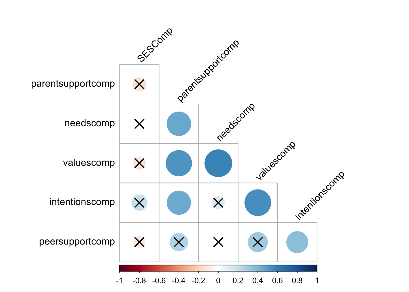
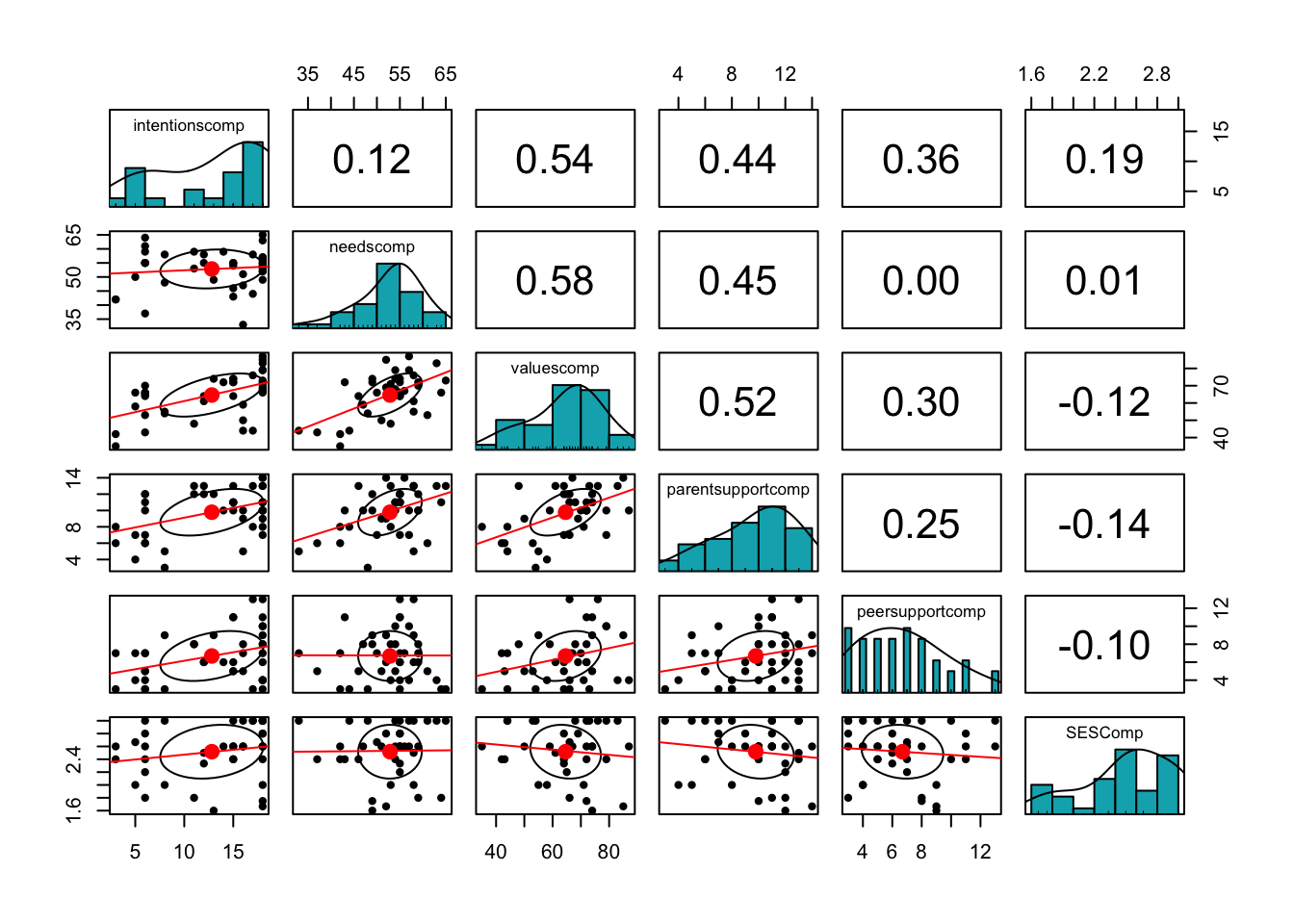
# Draw correlogram using psych
psych::pairs.panels(subsetdata,
method = "pearson", # correlation method
hist.col = "#00AFBB",
density = TRUE, # show density plots
ellipses = TRUE,
lm = TRUE# show correlation ellipses
)
# Automated reporting for statistical tests
report(cor.test(subsetdata$needscomp, subsetdata$valuescomp))## Effect sizes were labelled following Funder's (2019) recommendations.
##
## The Pearson's product-moment correlation between subsetdata$needscomp and
## subsetdata$valuescomp is positive, statistically significant, and very large (r
## = 0.58, 95% CI [0.33, 0.76], t(37) = 4.36, p < .001)6.3 Correlation vs. Causation
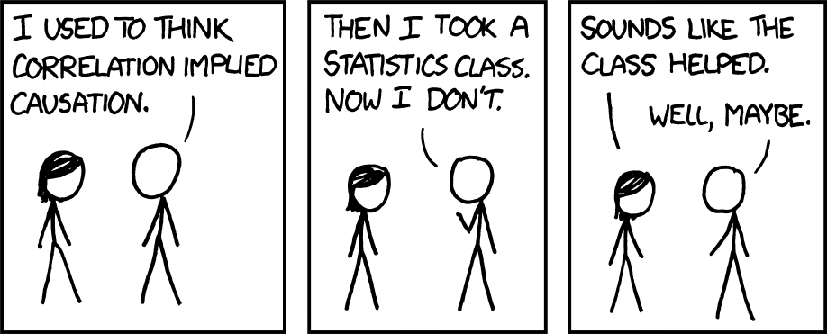
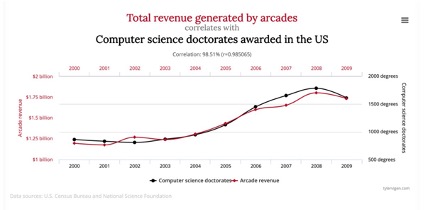
Correlation does not equal causation as finding a correlation between two variables does not establish a causal relationship. To establish causality, we need to know the underlying directionality/ordering of the relationship and rule out confounding variables that might explain the relationship (e.g., a strong positive correlation exists between total revenue generated by arcades and computer science doctorates awarded, However, one does not cause the other).
6.4 Cronbach’s Alpha—Reliability Estimates
Cronbach’s alpha is used to determine the internal consistency of a continuous scale or subscale and is computed by using correlations among the item scores included in the scale. There are other types of reliability (see Chapter 17 of the Russell Text), but we will focus on Cronbach’s as it helps us determine item-consistency across samples. Subscales can be deemed reliable at an alpha level above .70. Exploratory studies might use more liberal thresholds.
Music education researchers often use Cronbach’s alpha to help validate a scale or subscale of a test or research project. The scale if item deleted option provides a measure of reliability without certain items and can help us create a more consistent measure in pilot testing or in initial phases of analysis.
6.5 Correlational Analysis Practice
6.5.1 Research Scenarios
A college Dean questions whether music faculty who are promoted from Assistant Professor to Associate and Full Professor achieve a greater degree of visibility (regional, national, international).
a. Chi-Square
b. Spearman’s Rho
c. Pearson’s R
A high school choir director believes that ensemble rankings at a national show choir contest may be strongly related to the operating budget available to each choir.
a. Chi-Square
b. Spearman’s Rho
c. Pearson’s R
A music supervisor wants to know the number of students enrolled in music classes at middle schools within her district, and whether these participation rates are related to the number of instructional periods scheduled at each school.
a. Chi-Square
b. Spearman’s Rho
c. Pearson’s R
A university researcher conducts a national survey focused on string music education and wants to know whether the geographic region in which an institution is located has any relationship to whether the institution employs a string music educator on the faculty.
a. Chi-Square
b. Spearman’s Rho
c. Pearson’s R
A high school band director wants to know whether there is a relationship between number of years of private lesson instruction and the amount of weekly practice time.
a. Chi-Square
b. Spearman’s Rho
c. Pearson’s R
A department head has a hunch that more experienced music teachers are less motivated to engage in competitive music events.
a. Chi-Square
b. Spearman’s Rho
c. Pearson’s R
A beginning band director wants to know if there is a relationship between gender identity and the band instrument a student is most interested in playing.
a. Chi-Square
b. Spearman’s Rho
c. Pearson’s R
A middle school orchestra teacher wonders whether students playing 1st parts within each section are disproportionately of Asian and Caucasian backgrounds as compared to students playing 2nd parts.
a. Chi-Square
b. Spearman’s Rho
c. Pearson’s R
6.5.2 Data Analysis
6.5.2.1 Checking for Assumptions
install.packages("outliers")
install.packages("summarytools")
install.packages("ggstatsplot")
install.packages("outliers")
install.packages("skedastic")data <- read_excel('pearson_correlation_example_1.xlsx')
data## # A tibble: 40 × 2
## GPA PerformanceFinal
## <dbl> <dbl>
## 1 3.21 7
## 2 3.88 9
## 3 3.55 7
## 4 3.78 8
## 5 3.87 9
## 6 3.55 8
## 7 3.65 8
## 8 3.21 7
## 9 3.78 8
## 10 3.9 9
## # … with 30 more rowsAre data continuous? Analyses that use Pearson’s R must be conducted on continuous variables (e.g., scores out of 100). There is one exception—you can correlate a binary (yes/no, 0/1) variable with a continuous variable. This is called a Point-Biserial Correlation, but uses the same conventions and approach as Pearson’s R.
Are data normally distributed? The quickest way to check for normality is the Shapiro test, or you can take a quick glance at the skewness/kurtosis values using psych::describe(). You can also the summarytools package and the dfSummary() or descr() functions. If data are not normally distributed but you still prefer to use Pearson’s R, you can force a transformation of the data into a normal distribution using log() or log10().
library(summarytools)##
## Attaching package: 'summarytools'## The following object is masked from 'package:tibble':
##
## view# Summaries
dfSummary(data)## Data Frame Summary
## data
## Dimensions: 40 x 2
## Duplicates: 4
##
## ---------------------------------------------------------------------------------------------------------------
## No Variable Stats / Values Freqs (% of Valid) Graph Valid Missing
## ---- ------------------ ----------------------- -------------------- --------------------- ---------- ---------
## 1 GPA Mean (sd) : 3.1 (0.6) 34 distinct values : . 40 0
## [numeric] min < med < max: . : : (100.0%) (0.0%)
## 2.1 < 3 < 4 : : : : : : :
## IQR (CV) : 1.1 (0.2) : : : : : : . : :
## : : : : : : . : : :
##
## 2 PerformanceFinal Mean (sd) : 6.7 (1.6) 4 : 4 (10.0%) II 40 0
## [numeric] min < med < max: 5 : 7 (17.5%) III (100.0%) (0.0%)
## 4 < 7 < 9 6 : 8 (20.0%) IIII
## IQR (CV) : 3 (0.2) 7 : 7 (17.5%) III
## 8 : 8 (20.0%) IIII
## 9 : 6 (15.0%) III
## ---------------------------------------------------------------------------------------------------------------descr(data)## Descriptive Statistics
## data
## N: 40
##
## GPA PerformanceFinal
## ----------------- -------- ------------------
## Mean 3.09 6.65
## Std.Dev 0.61 1.59
## Min 2.11 4.00
## Q1 2.56 5.00
## Median 3.04 7.00
## Q3 3.67 8.00
## Max 4.00 9.00
## MAD 0.88 1.48
## IQR 1.11 3.00
## CV 0.20 0.24
## Skewness 0.02 -0.06
## SE.Skewness 0.37 0.37
## Kurtosis -1.48 -1.22
## N.Valid 40.00 40.00
## Pct.Valid 100.00 100.00create_report(data)##
##
## processing file: report.rmd##
|
| | 0%
|
|.. | 2%
## inline R code fragments
##
##
|
|... | 5%
## label: global_options (with options)
## List of 1
## $ include: logi FALSE
##
##
|
|..... | 7%
## ordinary text without R code
##
##
|
|....... | 10%
## label: introduce
##
|
|........ | 12%
## ordinary text without R code
##
##
|
|.......... | 14%
## label: plot_intro##
|
|............ | 17%
## ordinary text without R code
##
##
|
|............. | 19%
## label: data_structure
##
|
|............... | 21%
## ordinary text without R code
##
##
|
|................. | 24%
## label: missing_profile##
|
|.................. | 26%
## ordinary text without R code
##
##
|
|.................... | 29%
## label: univariate_distribution_header
##
|
|...................... | 31%
## ordinary text without R code
##
##
|
|....................... | 33%
## label: plot_histogram##
|
|......................... | 36%
## ordinary text without R code
##
##
|
|........................... | 38%
## label: plot_density
##
|
|............................ | 40%
## ordinary text without R code
##
##
|
|.............................. | 43%
## label: plot_frequency_bar
##
  |
  |................................                                      |  45%
##   ordinary text without R code
##
##
  |
  |.................................                                     |  48%
## label: plot_response_bar
##
  |
  |...................................                                   |  50%
##   ordinary text without R code
##
##
  |
  |.....................................                                 |  52%
## label: plot_with_bar
##
  |
  |......................................                                |  55%
##   ordinary text without R code
##
##
  |
  |........................................                              |  57%
## label: plot_normal_qq
##
|
|.......................................... | 60%
## ordinary text without R code
##
##
|
|........................................... | 62%
## label: plot_response_qq
##
|
|............................................. | 64%
## ordinary text without R code
##
##
|
|............................................... | 67%
## label: plot_by_qq
##
|
|................................................ | 69%
## ordinary text without R code
##
##
|
|.................................................. | 71%
## label: correlation_analysis##
|
|.................................................... | 74%
## ordinary text without R code
##
##
|
|..................................................... | 76%
## label: principal_component_analysis##
|
|....................................................... | 79%
## ordinary text without R code
##
##
|
|......................................................... | 81%
## label: bivariate_distribution_header
##
|
|.......................................................... | 83%
## ordinary text without R code
##
##
|
|............................................................ | 86%
## label: plot_response_boxplot
##
|
|.............................................................. | 88%
## ordinary text without R code
##
##
|
|............................................................... | 90%
## label: plot_by_boxplot
##
|
|................................................................. | 93%
## ordinary text without R code
##
##
|
|................................................................... | 95%
## label: plot_response_scatterplot
##
|
|.................................................................... | 98%
## ordinary text without R code
##
##
|
|......................................................................| 100%
## label: plot_by_scatterplot## output file: /Users/jbh6331/Desktop/R/540/report.knit.md## /Applications/RStudio.app/Contents/MacOS/quarto/bin/pandoc +RTS -K512m -RTS /Users/jbh6331/Desktop/R/540/report.knit.md --to html4 --from markdown+autolink_bare_uris+tex_math_single_backslash --output /Users/jbh6331/Desktop/R/540/report.html --lua-filter /Users/jbh6331/Library/R/x86_64/4.2/library/rmarkdown/rmarkdown/lua/pagebreak.lua --lua-filter /Users/jbh6331/Library/R/x86_64/4.2/library/rmarkdown/rmarkdown/lua/latex-div.lua --self-contained --variable bs3=TRUE --standalone --section-divs --table-of-contents --toc-depth 6 --template /Users/jbh6331/Library/R/x86_64/4.2/library/rmarkdown/rmd/h/default.html --no-highlight --variable highlightjs=1 --variable theme=yeti --mathjax --variable 'mathjax-url=https://mathjax.rstudio.com/latest/MathJax.js?config=TeX-AMS-MML_HTMLorMML' --include-in-header /var/folders/_t/4fctbs650sqbl5b86n88pnbdb8jsl9/T//RtmpUInMZ0/rmarkdown-str183db37828eb1.html##
## Output created: report.html# Shapiro-Wilk
data %>% shapiro_test(GPA, PerformanceFinal)## # A tibble: 2 × 3
## variable statistic p
## <chr> <dbl> <dbl>
## 1 GPA 0.923 0.00976
## 2 PerformanceFinal 0.924 0.00994# Kolmogorov-Smirnov
ks.test(data$PerformanceFinal, "pnorm")## Warning in ks.test.default(data$PerformanceFinal, "pnorm"): ties should not be
## present for the Kolmogorov-Smirnov test##
## Asymptotic one-sample Kolmogorov-Smirnov test
##
## data: data$PerformanceFinal
## D = 0.99997, p-value < 2.2e-16
## alternative hypothesis: two-sided#Transformed with log
data$GPAlog <- log(data$GPA)
data$PerformanceFinallog <- log10(data$PerformanceFinal)
data %>% shapiro_test(PerformanceFinal, PerformanceFinallog)## # A tibble: 2 × 3
## variable statistic p
## <chr> <dbl> <dbl>
## 1 PerformanceFinal 0.924 0.00994
## 2 PerformanceFinallog 0.914 0.00484Do analyzed data contain any outliers?
# tag outliers with ggstatsplot
library(ggstatsplot)
## You can cite this package as:
## Patil, I. (2021). Visualizations with statistical details: The 'ggstatsplot' approach.
## Journal of Open Source Software, 6(61), 3167, doi:10.21105/joss.03167##
## Attaching package: 'ggstatsplot'## The following object is masked from 'package:data.table':
##
## :=ggscatterstats(data, GPA, PerformanceFinal, outlier.tagging = TRUE)## Registered S3 method overwritten by 'ggside':
## method from
## +.gg ggplot2## `stat_bin()` using `bins = 30`. Pick better value with `binwidth`.
## `stat_bin()` using `bins = 30`. Pick better value with `binwidth`.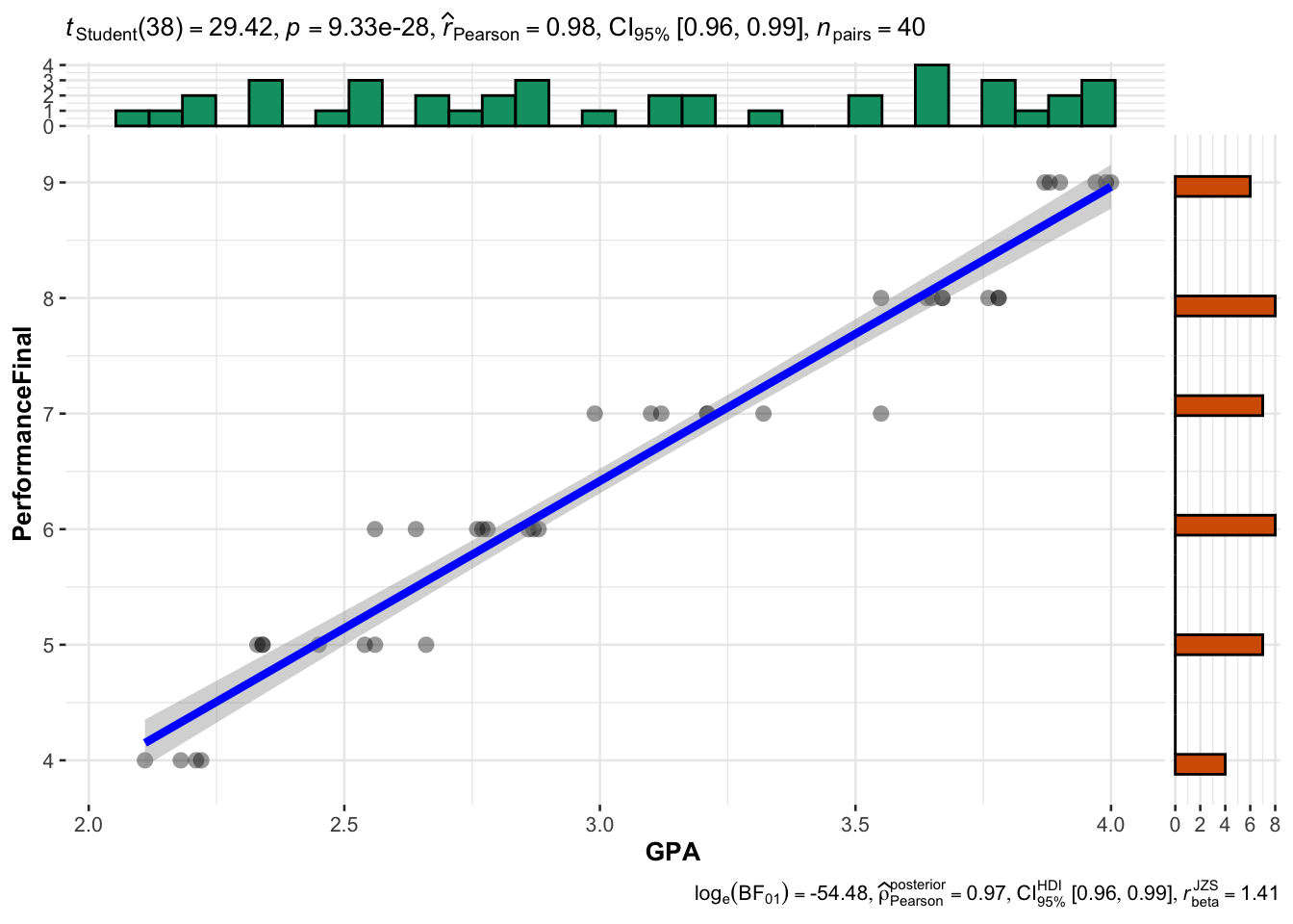
library(outliers)##
## Attaching package: 'outliers'## The following object is masked from 'package:psych':
##
## outlierboxplot(data$GPA, plot=F)$out## numeric(0)data <- data[data$GPA > 2.18, ] Are relationships between data linear? There should be a clear direct or indirect relationship, be it weak, in the scatterplot.
plot(GPA ~ PerformanceFinal, data = data, main = 'Relationship Between GPA and Performance')
abline(lm(data$GPA ~ data$PerformanceFinal))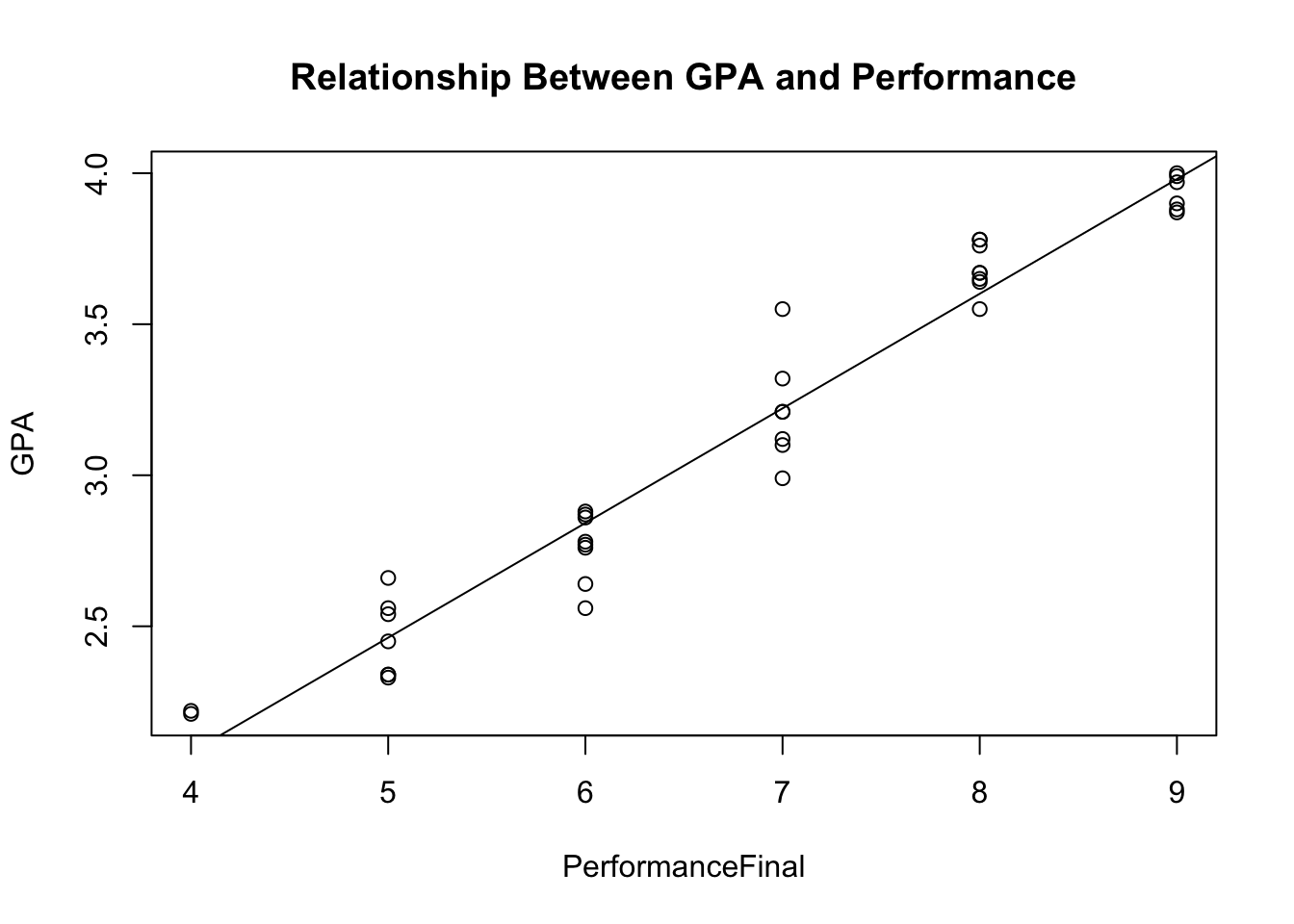
Does the data have homoscedasticity? Put otherwise, do the data vary at similar rates across the range of responses? A scatterplot check will suffice here, as well, but if you want a test to make sure, see below.
library(skedastic)
model <- lm(GPA ~ PerformanceFinal, data = data)
skedastic::white_lm(model)
## # A tibble: 1 × 5
## statistic p.value parameter method alternative
## <dbl> <dbl> <dbl> <chr> <chr>
## 1 2.16 0.340 2 White's Test greater6.5.2.2 Pearson’s R
We do: Russell p. 52 (Pearson Example 1 Dataset). Follow instructions on this page to complete the same test in SPSS.
data %>% cor_test(GPA, PerformanceFinal, method = 'pearson')## # A tibble: 1 × 8
## var1 var2 cor statistic p conf.low conf.high method
## <chr> <chr> <dbl> <dbl> <dbl> <dbl> <dbl> <chr>
## 1 GPA PerformanceFinal 0.98 26.8 2.13e-25 0.954 0.988 Pearsonx <- cor.test(data$GPA, data$PerformanceFinal)
report(x)## Effect sizes were labelled following Funder's (2019) recommendations.
##
## The Pearson's product-moment correlation between data$GPA and
## data$PerformanceFinal is positive, statistically significant, and very large (r
## = 0.98, 95% CI [0.95, 0.99], t(36) = 26.84, p < .001)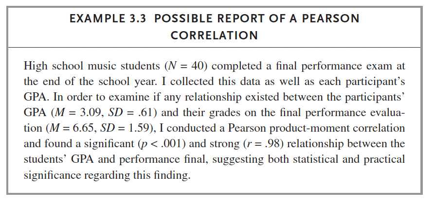
You do: Russell p. 58 (Pearson Example 2 Dataset) using either SPSS or R and produce short write up of results.
library(readxl)
data <- read_excel('pearson_correlation_example_2.xlsx')
data$TeachingEffective <- data$TeachingEffecitve
data <- data %>% select(-TeachingEffecitve)

#cor.test(data$TeachingExperience, data$TeachingJoy)
6.5.2.3 Chi-Square
We do: Russell p. 259 (Chi-Square Example 1 Dataset). Follow instructions on this page to complete the same test in SPSS.
data <- read_excel('chi_square_example_1.xlsx')
table(data$InstrumentType, data$PersonalityType)
##
## 1 2
## 1 45 16
## 2 43 33chisq.test(data$InstrumentType, data$PersonalityType)##
## Pearson's Chi-squared test with Yates' continuity correction
##
## data: data$InstrumentType and data$PersonalityType
## X-squared = 3.6371, df = 1, p-value = 0.0565chisq_test(data$InstrumentType, data$PersonalityType)## # A tibble: 1 × 6
## n statistic p df method p.signif
## * <int> <dbl> <dbl> <int> <chr> <chr>
## 1 137 3.64 0.0565 1 Chi-square test ns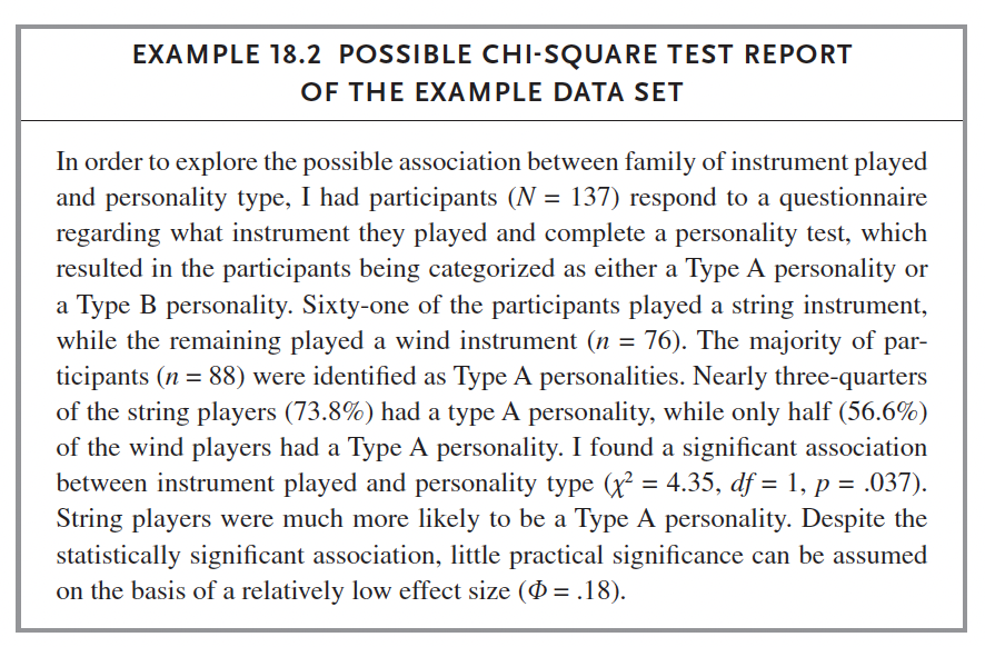
You do: Russell p. 267 (Chi-Square Example 2 Dataset) using SPSS or R and produce short write up of results.
6.5.2.4 Spearman’s Rho
We do: Russell p. 295 (Spearman Example 1 Dataset). Follow instructions on this page to complete the same test in SPSS.
data <- read_excel('spearman_example_1.xlsx')
data %>% cor_test(ConductExpress, PerformExpress, method = 'spearman')
## # A tibble: 1 × 6
## var1 var2 cor statistic p method
## <chr> <chr> <dbl> <dbl> <dbl> <chr>
## 1 ConductExpress PerformExpress 0.4 37317. 0.000499 Spearmanx <- cor.test(data$ConductExpress, data$PerformExpress, method = 'spearman')## Warning in cor.test.default(data$ConductExpress, data$PerformExpress, method =
## "spearman"): Cannot compute exact p-value with tiesreport(x)## Effect sizes were labelled following Funder's (2019) recommendations.
##
## The Spearman's rank correlation rho between data$ConductExpress and
## data$PerformExpress is positive, statistically significant, and very large (rho
## = 0.40, S = 37316.63, p < .001)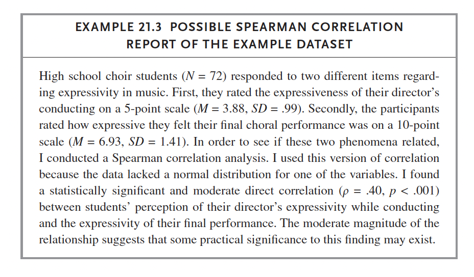
You do: Russell p. 297 (Spearman Example 2 Dataset) using SPSS or R and produce short write up of results.
6.5.2.5 Cronbach’s Alpha
We do: Russell p. 241 (Cronbach’s Example 1 Dataset). Follow instructions on this page to complete this test in SPSS.
data <- read_excel('cronbachs_alpha_example_1.xlsx')
data$popmusician <- as.numeric(data$popmusician)
## Warning: NAs introduced by coerciondata$conductfac <- as.numeric(data$conductfac)## Warning: NAs introduced by coerciondata$msmusicteach <- as.numeric(data$msmusicteach)## Warning: NAs introduced by coercionalpha(data)##
## Reliability analysis
## Call: alpha(x = data)
##
## raw_alpha std.alpha G6(smc) average_r S/N ase mean sd median_r
## 0.78 0.79 0.83 0.32 3.8 0.031 4.1 0.52 0.35
##
## 95% confidence boundaries
## lower alpha upper
## Feldt 0.71 0.78 0.83
## Duhachek 0.72 0.78 0.84
##
## Reliability if an item is dropped:
## raw_alpha std.alpha G6(smc) average_r S/N alpha se var.r med.r
## elementteach 0.78 0.79 0.82 0.36 3.9 0.031 0.039 0.37
## popmusician 0.82 0.82 0.84 0.40 4.7 0.026 0.026 0.39
## conductfac 0.74 0.76 0.80 0.31 3.1 0.037 0.046 0.33
## classicmusician 0.75 0.77 0.80 0.32 3.3 0.036 0.049 0.37
## hsmusicteach 0.73 0.74 0.77 0.29 2.9 0.038 0.041 0.33
## appliedfac 0.72 0.74 0.78 0.29 2.9 0.039 0.042 0.33
## msmusicteach 0.72 0.74 0.76 0.29 2.9 0.039 0.038 0.33
## musicedfac 0.76 0.77 0.81 0.33 3.4 0.035 0.048 0.34
##
## Item statistics
## n raw.r std.r r.cor r.drop mean sd
## elementteach 118 0.51 0.51 0.42 0.33 4.4 0.92
## popmusician 116 0.35 0.32 0.17 0.14 3.5 0.96
## conductfac 117 0.70 0.70 0.65 0.57 3.9 0.88
## classicmusician 118 0.66 0.65 0.58 0.52 3.9 0.85
## hsmusicteach 118 0.76 0.77 0.77 0.67 4.4 0.70
## appliedfac 118 0.77 0.77 0.75 0.66 4.3 0.81
## msmusicteach 116 0.76 0.77 0.78 0.66 4.2 0.86
## musicedfac 118 0.59 0.61 0.53 0.46 4.4 0.70
##
## Non missing response frequency for each item
## 1 2 3 4 5 miss
## elementteach 0.02 0.04 0.08 0.30 0.57 0.00
## popmusician 0.00 0.16 0.35 0.31 0.18 0.02
## conductfac 0.00 0.05 0.26 0.38 0.31 0.01
## classicmusician 0.01 0.04 0.23 0.47 0.25 0.00
## hsmusicteach 0.01 0.00 0.07 0.40 0.53 0.00
## appliedfac 0.00 0.03 0.13 0.37 0.47 0.00
## msmusicteach 0.01 0.02 0.20 0.36 0.41 0.02
## musicedfac 0.00 0.01 0.09 0.36 0.54 0.00nopopdata <- data %>% select(-popmusician)
alpha(nopopdata)##
## Reliability analysis
## Call: alpha(x = nopopdata)
##
## raw_alpha std.alpha G6(smc) average_r S/N ase mean sd median_r
## 0.82 0.82 0.84 0.4 4.7 0.026 4.2 0.57 0.39
##
## 95% confidence boundaries
## lower alpha upper
## Feldt 0.76 0.82 0.86
## Duhachek 0.77 0.82 0.87
##
## Reliability if an item is dropped:
## raw_alpha std.alpha G6(smc) average_r S/N alpha se var.r med.r
## elementteach 0.83 0.83 0.84 0.45 4.9 0.025 0.018 0.45
## conductfac 0.79 0.80 0.82 0.40 3.9 0.030 0.029 0.39
## classicmusician 0.81 0.82 0.83 0.43 4.5 0.027 0.024 0.44
## hsmusicteach 0.78 0.78 0.79 0.37 3.5 0.033 0.026 0.37
## appliedfac 0.77 0.78 0.80 0.37 3.6 0.032 0.026 0.37
## msmusicteach 0.77 0.78 0.78 0.37 3.5 0.034 0.025 0.37
## musicedfac 0.80 0.81 0.83 0.42 4.3 0.029 0.034 0.47
##
## Item statistics
## n raw.r std.r r.cor r.drop mean sd
## elementteach 118 0.57 0.55 0.45 0.38 4.4 0.92
## conductfac 117 0.71 0.71 0.65 0.58 3.9 0.88
## classicmusician 118 0.61 0.61 0.51 0.45 3.9 0.85
## hsmusicteach 118 0.78 0.79 0.77 0.69 4.4 0.70
## appliedfac 118 0.77 0.78 0.75 0.67 4.3 0.81
## msmusicteach 116 0.80 0.80 0.80 0.70 4.2 0.86
## musicedfac 118 0.63 0.65 0.55 0.51 4.4 0.70
##
## Non missing response frequency for each item
## 1 2 3 4 5 miss
## elementteach 0.02 0.04 0.08 0.30 0.57 0.00
## conductfac 0.00 0.05 0.26 0.38 0.31 0.01
## classicmusician 0.01 0.04 0.23 0.47 0.25 0.00
## hsmusicteach 0.01 0.00 0.07 0.40 0.53 0.00
## appliedfac 0.00 0.03 0.13 0.37 0.47 0.00
## msmusicteach 0.01 0.02 0.20 0.36 0.41 0.02
## musicedfac 0.00 0.01 0.09 0.36 0.54 0.00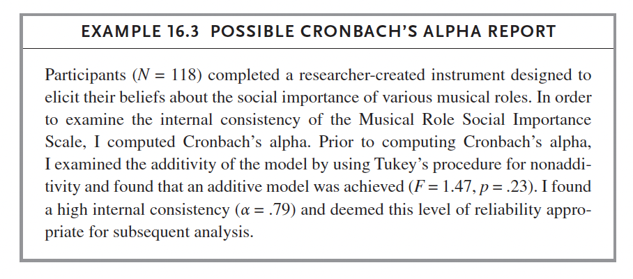
You do: Russell p. 245 (Cronbach’s Example 2 Dataset) in SPSS or R and produce short write up of results.