2 Problem Identification and Descriptive Statistics (8/24)
Share Out Articles: focus on problem the authors are attempting to address and whether you feel they were successful or not.
Algorithm Reading Quiz: build familiarity with a simple statistical method.
Hypotheses: Null, alternative, directional, and research questions.
99 Problems (but my method ain’t one) : Your project officially starts here.
Descriptive Stats: Doing and interpreting measures of central tendency and variability.
Due Next Time: Read and present descriptive statistics on one Quantitative JRME article. Download SPSS, R, and R Studio. Launch SPSS, and R Studio to make sure they both are working.
Examine the symbols in this image and email me the answer when you know what the algorithm represents. Googling, or referencing the Russell text is allowed.
2.1 Hypotheses and Research Questions
A hypothesis is a proposed solution to a problem. To test a hypothesis is to take a rational (logical) decision based on observed data. In music education, hypotheses tend to have an underlying goal of _____________________?
After formulating some hypothesis (e.g., there is no difference in the performance ability between 6th and 7th grade band students) we collect and interpret data to either accept or reject the null hypothesis (h0), or the post-positivistic assumption that there is no difference between 6th and 7th graders, and that the intention of the research conducted is to disprove that assumption.
Alternative hypotheses (h1) simply assume the opposite (i.e., there is a difference between 6th and 7th graders). A directional hypothesis assumes that one outcome will be decidedly different, for instance in one direction (e.g., 7th graders have a higher performance ability than 6th graders). Alternate and directional hypotheses do not threaten our post-positivistic viewpoints, if the notions of a null hypothesis are implicit, and the researcher is willing to accept the lack of an effect.
Or, consider the following meme.

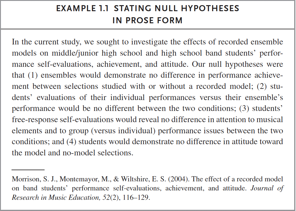
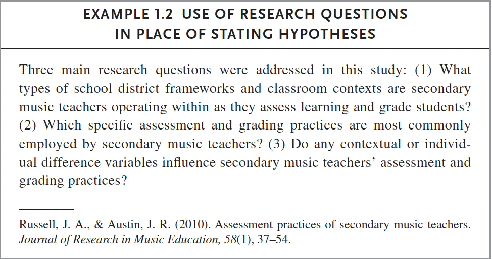
You can also state the null or alternative hypothesis in the form of a research question, this is commonly accepted in publications.
Identify two problem areas that you want to address with research in this class. See if you can answer these questions with one to two sentences, without accessing resources.
Why does this problem need to be addressed?
How have others tried to address the problem?
What do you know and not know about the problem?
What is a hypothesis that you have regarding this problem?
Can you restate your hypothesis in the form of a research question?
2.2 Descriptive Statistics
Descriptive statistics provide a (for lack of a better term) description of what is observed in collected data—whereby measures of centrality and variability are our main tools for understanding. These are oftentimes referred to as summary statistics. We use descriptive statistics to assess the characteristics of participants, which supports the ability to make statements regarding make the generalizability of the sample to the overall population or other context.
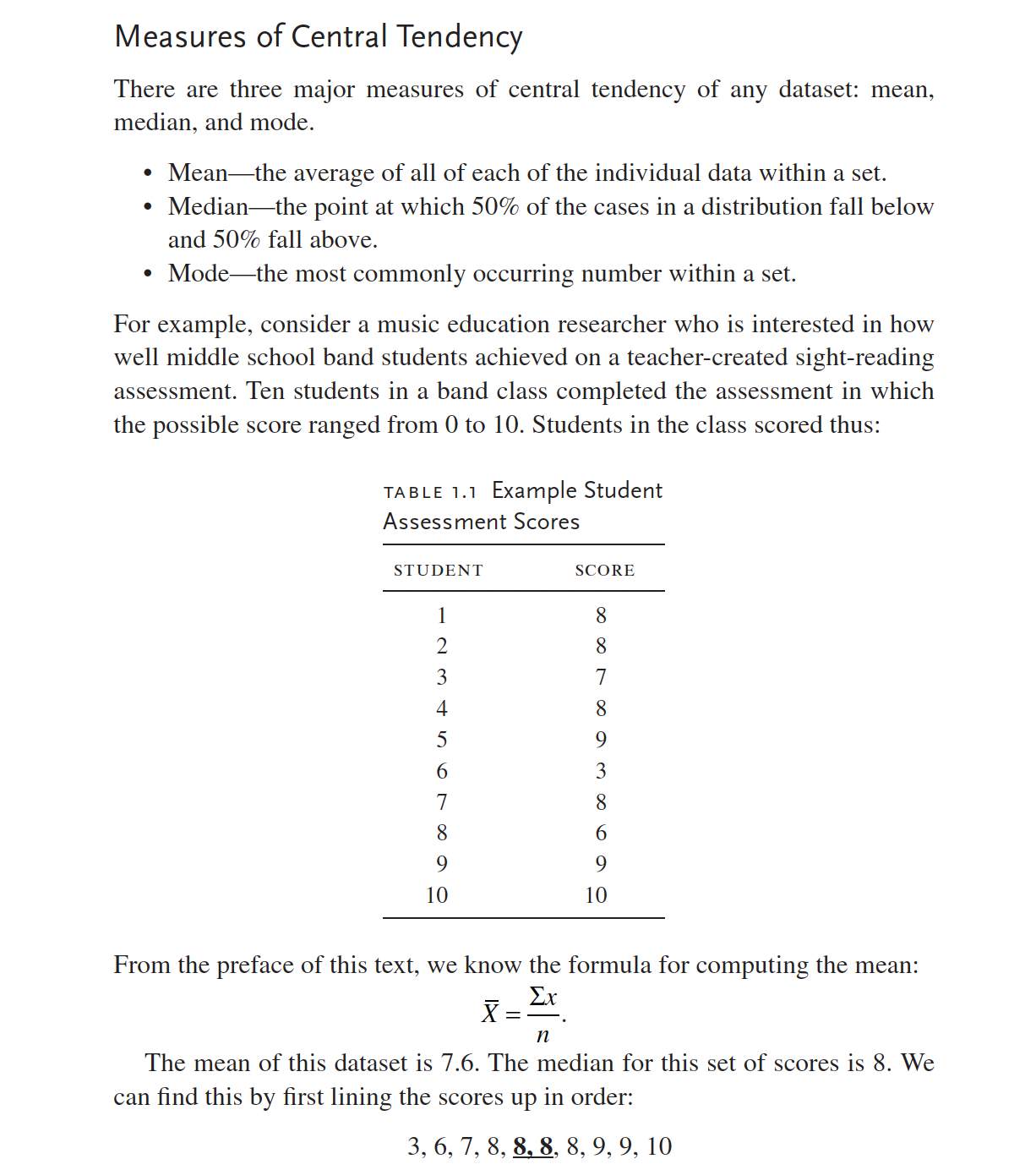
Measures of central tendency are used to describe data with a single number. For instance, the mean represents the average of all of each of the individual data within a set. See the following example from the first Russell chapter:
2.2.1 A Non-Music Education Example
We are going to utilize the mtcars dataset to apply descriptive statistical concepts using R. The dataset includes information regarding fuel consumption and 10 other aspects of automobile design and performance across 32 automobiles.
Put otherwise, mtcars is a data frame with 32 observations of 11 (numeric) variables. These include:
Miles/(US) gallon (mpg)
Number of cylinders (cyl)
Displacement (disp)
Gross horsepower (hp)
Rear axle ratio (drat)
Weight in 1000 lbs (wt)
1/4 mile time (qsec)
Engine (0 = V-shaped, 1 = straight) (vs)
Transmission (0 = automatic, 1 = manual) (am)
Number of forward gears (gear)
Number of carburetors (carb)
library(tidyverse)## ── Attaching packages ─────────────────────────────────────── tidyverse 1.3.2 ──
## ✔ ggplot2 3.3.6 ✔ purrr 0.3.5
## ✔ tibble 3.1.8 ✔ dplyr 1.0.10
## ✔ tidyr 1.2.1 ✔ stringr 1.4.0
## ✔ readr 2.1.2 ✔ forcats 0.5.1
## ── Conflicts ────────────────────────────────────────── tidyverse_conflicts() ──
## ✖ dplyr::filter() masks stats::filter()
## ✖ dplyr::lag() masks stats::lag()library(psych)##
## Attaching package: 'psych'
##
## The following objects are masked from 'package:ggplot2':
##
## %+%, alpha#View(mtcars)mean(mtcars$mpg)## [1] 20.09062mean(mtcars$mpg)## [1] 20.09062The median describes the point at which 50% of cases in a distribution fall below and 50% fall above.
median(mtcars$mpg)## [1] 19.2Variability is the amount of spread or dispersion in a set of scores. Knowing the extent to which data varies allows researchers to compare groups within data effectively and accurately.
Assessments of variability provide a representation of the amount of dispersion within a distribution from a measure of central tendency. For instance, range displays the lowest and highest score in a vector.
range(mtcars$mpg)## [1] 10.4 33.9Standard deviation represents the average score deviation from the mean.
sd(mtcars$mpg)## [1] 6.026948Variance is the square of the standard deviation.
var(mtcars$mpg)## [1] 36.3241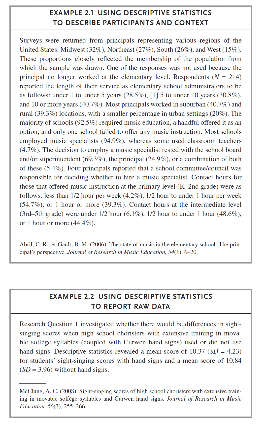
In reference to the distribution of the data, standard deviations tell us where scores generally fall. SD is often reported alongside the mean (e.g., M = 7, SD = 1.5). With these numbers, we can ascertain that 68% of scores will fall between 5.5 and 8.5, and 95% of scores fall between 4 and 10. Furthermore, we can ascertain with a normal distribution that about 99% of scores might fall between 2.5 and 12.5.
These association between means, standard deviations, and normal distributions parameterize the probability of future observations on a similar measure. Many of the most common statistical tests we use are conceived of assuming this parametric concept—rationalizing the assumption that observations will be normally distributed.
As exemplified above, data that meet this assumption tend to have around 68% of data points falling between +-1 standard deviation of the mean, and 95% of data falling between +-2 standard deviations of the mean. Furthermore, normality tends to be met when the distribution curve is peaked at the mean and has only one mode. Additionally, the curve in a normal distribution should be symmetrical on both sides of the mean, median, and mode while having asymptotic tails (tails curve but do not approach the axis; no 100s or zeros).
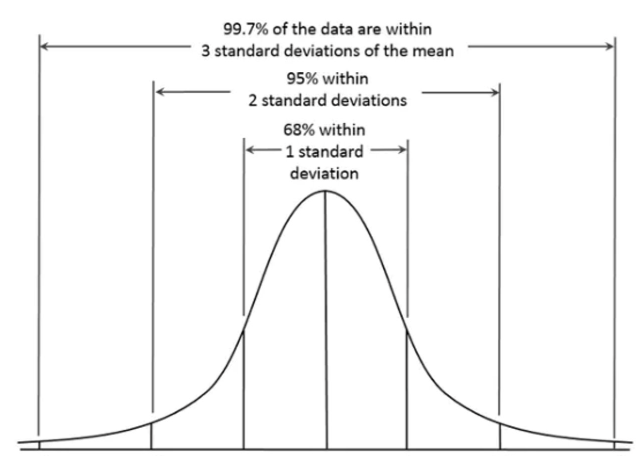
A distribution is skewed, or has skewness, positively or negatively when there is longer tail on one of the distribution. A longer tail on the right tends to indicate a smaller number of data points at the higher end of the distribution—a positive skew. A shorter tail on the right indicates a larger number of data points on the high end of the distribution—a negative skew.
One helpful rule of thumb is that if the mean is greater than the median the distribution likely has a positive skew. Conversely, if the mean is less than the median, the distribution likely has a negative skew. See the figure below for an illustration of each distribution.
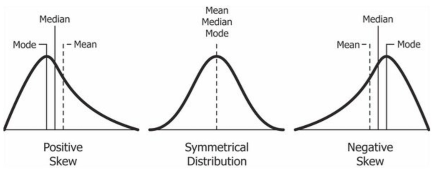
The smaller the standard deviation and variance, the higher the level of agreement, or similarity, in response or scores. When agreement or similarity in scores is very high a distribution may be leptokurtic—having low variance (i.e., small standard deviations). When scores are very broad high variance may create a platykurtic distribution. These are represented within the concept of kurtosis. Kurtosis will be assessed alongside skewness in a few paragraphs.
There are several ways to assess for the assumption of normality. Some researchers prefer to visually assess histograms. Some like to compare means and medians within the context of standard deviations. The most reliable, and mathematically-based, may be a Shapiro-Wilk test. A non-significant Shapiro-Wilk outcome will provide support of a normal distribution as test significance can be practically interpreted to suggest that the distribution is significantly different than a vector that is normally distributed. For instance, as the p value exceeds .05 when applied to the mtcars mpg column the miles per gallon variable can be interpreted as normally distributed across the vector. Use the function shapiro.test()
shapiro.test(mtcars$mpg)##
## Shapiro-Wilk normality test
##
## data: mtcars$mpg
## W = 0.94756, p-value = 0.1229You can also examine the influence of kurtosis and skewness values using the psych::describe() function. Interpretations of skewness and kurtosis values differ from field to field, but generally you can assume a normal distribution if these values fall within -3 and +3.
psych::describe(mtcars$mpg)## vars n mean sd median trimmed mad min max range skew kurtosis se
## X1 1 32 20.09 6.03 19.2 19.7 5.41 10.4 33.9 23.5 0.61 -0.37 1.07Use the psych function describeBy() and the argument group to see summary statistics grouped by any variable. The code below groups by transmission, where automatic = 0 and manual = 1). The use of double colons :: tells R to use the function from this specific package and not any other describeBy() function from packages other than psych.
psych::describeBy(mtcars, group='am') # summary statistics by grouping variable##
## Descriptive statistics by group
## am: 0
## vars n mean sd median trimmed mad min max range skew
## mpg 1 19 17.15 3.83 17.30 17.12 3.11 10.40 24.40 14.00 0.01
## cyl 2 19 6.95 1.54 8.00 7.06 0.00 4.00 8.00 4.00 -0.95
## disp 3 19 290.38 110.17 275.80 289.71 124.83 120.10 472.00 351.90 0.05
## hp 4 19 160.26 53.91 175.00 161.06 77.10 62.00 245.00 183.00 -0.01
## drat 5 19 3.29 0.39 3.15 3.28 0.22 2.76 3.92 1.16 0.50
## wt 6 19 3.77 0.78 3.52 3.75 0.45 2.46 5.42 2.96 0.98
## qsec 7 19 18.18 1.75 17.82 18.07 1.19 15.41 22.90 7.49 0.85
## vs 8 19 0.37 0.50 0.00 0.35 0.00 0.00 1.00 1.00 0.50
## am 9 19 0.00 0.00 0.00 0.00 0.00 0.00 0.00 0.00 NaN
## gear 10 19 3.21 0.42 3.00 3.18 0.00 3.00 4.00 1.00 1.31
## carb 11 19 2.74 1.15 3.00 2.76 1.48 1.00 4.00 3.00 -0.14
## kurtosis se
## mpg -0.80 0.88
## cyl -0.74 0.35
## disp -1.26 25.28
## hp -1.21 12.37
## drat -1.30 0.09
## wt 0.14 0.18
## qsec 0.55 0.40
## vs -1.84 0.11
## am NaN 0.00
## gear -0.29 0.10
## carb -1.57 0.26
## ------------------------------------------------------------
## am: 1
## vars n mean sd median trimmed mad min max range skew
## mpg 1 13 24.39 6.17 22.80 24.38 6.67 15.00 33.90 18.90 0.05
## cyl 2 13 5.08 1.55 4.00 4.91 0.00 4.00 8.00 4.00 0.87
## disp 3 13 143.53 87.20 120.30 131.25 58.86 71.10 351.00 279.90 1.33
## hp 4 13 126.85 84.06 109.00 114.73 63.75 52.00 335.00 283.00 1.36
## drat 5 13 4.05 0.36 4.08 4.02 0.27 3.54 4.93 1.39 0.79
## wt 6 13 2.41 0.62 2.32 2.39 0.68 1.51 3.57 2.06 0.21
## qsec 7 13 17.36 1.79 17.02 17.39 2.34 14.50 19.90 5.40 -0.23
## vs 8 13 0.54 0.52 1.00 0.55 0.00 0.00 1.00 1.00 -0.14
## am 9 13 1.00 0.00 1.00 1.00 0.00 1.00 1.00 0.00 NaN
## gear 10 13 4.38 0.51 4.00 4.36 0.00 4.00 5.00 1.00 0.42
## carb 11 13 2.92 2.18 2.00 2.64 1.48 1.00 8.00 7.00 0.98
## kurtosis se
## mpg -1.46 1.71
## cyl -0.90 0.43
## disp 0.40 24.19
## hp 0.56 23.31
## drat 0.21 0.10
## wt -1.17 0.17
## qsec -1.42 0.50
## vs -2.13 0.14
## am NaN 0.00
## gear -1.96 0.14
## carb -0.21 0.60Analyze frequency or count data for various groups using the table() function. The first line of code will create a table of counts disaggregated by transmission type and number of gears. The second line of code modifies the mtcars object to be grouped by transmission and gear, then summarizes each into a proportion of the entire population of cars as column ‘prop’ The spread() function is used to display the data of interest based on established groups.
table(mtcars$am, mtcars$gear)##
## 3 4 5
## 0 15 4 0
## 1 0 8 5mtcars %>% group_by(am, gear) %>% summarise(prop = n()/nrow(mtcars)) %>% spread(gear, prop)## `summarise()` has grouped output by 'am'. You can override using the `.groups`
## argument.## # A tibble: 2 × 4
## # Groups: am [2]
## am `3` `4` `5`
## <dbl> <dbl> <dbl> <dbl>
## 1 0 0.469 0.125 NA
## 2 1 NA 0.25 0.1562.2.2 A Music Education Example
data <- read_csv('participationdatashort.csv') # bring the dataset into environment
data
## # A tibble: 42 × 9
## intentionscomp needscomp value…¹ paren…² peers…³ SESComp Grade…⁴ Class Gender
## <dbl> <dbl> <dbl> <dbl> <dbl> <dbl> <chr> <chr> <chr>
## 1 8 58 55 5 9 2 eighth… band Male
## 2 18 54 79 10 10 2.4 sevent… orch… Female
## 3 6 61 53 6 5 3 sevent… band Female
## 4 15 55 72 11 6 3 sevent… orch… Female
## 5 16 47 59 10 8 2.6 sevent… band Male
## 6 17 58 76 13 13 3 sevent… band Male
## 7 18 54 68 11 8 3 sevent… band Female
## 8 6 37 43 6 5 2.4 sevent… band Female
## 9 16 33 44 5 7 3 sevent… orch… Male
## 10 3 42 42 6 7 2.4 eighth… band Female
## # … with 32 more rows, and abbreviated variable names ¹valuescomp,
## # ²parentsupportcomp, ³peersupportcomp, ⁴GradeLevelCalculate the mean and standard deviation of the variable “intentionscomp” as labelled in the dataset.
What do these values tell you about the elective intentionality of this sample, considering the possible points were 3-18.
Are these data normally and symmetrically distributed?
Link to full study: https://doi-org.ezaccess.libraries.psu.edu/10.1177/03057356221098095