3 Reading and Doing Descriptive Statistics (8/29)
Share out JRME article: Focus on descriptive statistics that you can identify and give a shot at interpreting them for us.
A quick R overview
Statistics review in practice: Mean, median, standard deviation, skewness, kurtosis.
Frequency distributions
Intro to data types and implications
Practice in R and SPSS
Due: Muijs Chapter 4 reading
Optional: Descriptive stats practice quiz is due next class if you want feedback.
3.1 The Integrated Development Environment
Where R is a programming language, RStudio is an integrated development environment (IDE) which enables users to efficiently access and view most facets of the program in a four pane environment. These include the source, console, environment and history, as well as the files, plots, packages and help. The console is in the lower-left corner, and this is where commands are entered and output is printed. The source pane is in the upper-left corner, and is a built in text editor. While the console is where commands are entered, the source pane includes executable code which communicates with the console. The environment tab, in the upper-right corner displays an list of loaded R objects. The history tab tracks the user’s keystrokes entered into the console. Tabs to view plots, packages, help, and output viewer tabs are in the lower-right corner.
Where SPSS and other menu based analytic software are limited by user input and installed software features, R operates as a mediator between user inputs and open source developments from our colleagues all over the world. This affords R users a certain flexibility. However, it takes a few extra steps to appropriately launch projects. Regardless of your needs with R, you will likely interact with the following elements of document set up.
3.1.1 Set Your Working Directory
It is helpful to use a project specific directory and to frequently save your work. When you first use R follow this procedure: Create a sub-directory (folder), “R” for example, in your “Documents” folder, or somewhere on your machine that you can easily access. This sub-folder, also known as working directory, will be used by R to read and save files. Think of it as a download and upload folder for R only.
You can specify your working directory to R in a few ways. One option is to click the "Session" drop down menu at the top of your screen and then click "Set Working Directory." It might also be useful to change the directory using code. To do this, use the function setwd(), and then enter the path of your directory into the parenthesis. Your working directory path will look something like what you see below. If you are unsure about the path you should input here, find the folder using your machine’s finder function, right click the folder, and examine the details of the folder’s path. Make sure that you are using forward slashes in quotes as the example indicates.
You will need to run the code chunk in order to process the change in working directory. To run a code chunk, you can select the code you want to run and hit command and enter simultaneously on Mac, or control and enter on a Windows machine. Alternatively, you can click the green play button in the top right corner of the code chunk to run the entire cell.
setwd('/Users/username/Desktop/R/')3.2 What do we measure, though?
Descriptive statistics, like all statistics, are derived from samples of larger populations. They provide a (for lack of a better term) description of what is observed in collected data—whereby means, medians, standard deviations, kurtosis, and skewness, are our main tools for understanding. These are oftentimes referred to as summary statistics, which gets at what they tend to do for researchers—summarize the qualities of a sample.
We tend to measure:
Sample characteristics (e.g., age, grade level, gender identification, family structure)
Behaviors (e.g., practice time, eye movements, what else?)
Constructs (I.e., organizing trait related to a behavior)
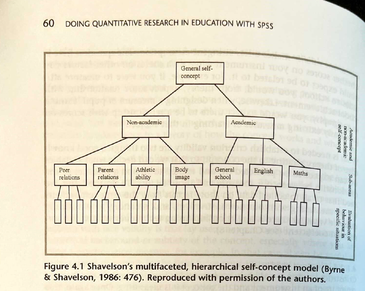
Constructs are the building blocks of theories. We use constructs to organize realms of knowledge that are measurable—striving to convert subjective experiences (e.g., qualities of peer and parent relationships) into objective patterns of behaviors (e.g., non-academic self-concept) in support of larger behavioral theories and research areas (e.g., self-concept predicts student valuation of music learning experiences). See this example from your reading that is due on Wednesday.
Let’s think together: What are some behaviors that might lend themselves to larger constructs? These could be based in research or on your own experiences (e.g., when x and y happened, students tended to ___).
3.2.1 Frequency Distributions
Frequency distributions include a list, table, or graph that displays the frequency of various outcomes in a sample. We learn about them because they bridge the gap between the concepts of descriptive statistics and data collection.
For instance, in a quantitative research methods course a survey was given. One question asked “where were you born?” A frequency distribution was then created based on the responses:
Southwest US: I I I
Southeast US: I I I I
Northeast US: I I I I I I
Northwest US: I I I I I
Outside of US: I I
Can you, or should you, calculate the mean? Median? Mode? % of students at each score level? Can we discuss variability (SD/kurtosis/etc.?) What if the same data were scores on a test?
Score 0:
Score 20: I I I
Score 40: I I I I
Score 60: I I I I I I
Score 80: I I I I I
Score 100: I I
Let’s import this dataset and do some descriptive statistics with it.
library(tidyverse)
data <- read_csv('frequencydistribution.csv')
## Rows: 20 Columns: 1
## ── Column specification ────────────────────────────────────────────────────────
## Delimiter: ","
## dbl (1): Scores
##
## ℹ Use `spec()` to retrieve the full column specification for this data.
## ℹ Specify the column types or set `show_col_types = FALSE` to quiet this message.#View(data)Calculate the mean using the function “mean()” and the arguments data$Scores
mean(data$Scores)## [1] 59Calculate the median using “median()”
median(data$Scores)## [1] 60Calculate the range using “range()”
range(data$Scores)## [1] 20 100Calculate the standard deviation using “sd()”
sd(data$Scores)## [1] 24.68752We need the package “moments” to calculate skewness and kurtosis.
install.packages('moments')Now we can keep rolling:
library(moments)
skewness(data$Scores)
## [1] -0.07622662kurtosis(data$Scores)## [1] 2.100808The skewness value should be between -2 and +2, and the kurtosis value should be between -7 and +7 to indicate a normal distribution (Bryne, 2010).
Alternatively, we can use the psych library and function psych::describe() to attain all of these values at once.
#install.packages("psych")
library(psych)
psych::describe(data$Scores)
## vars n mean sd median trimmed mad min max range skew kurtosis se
## X1 1 20 59 24.69 60 58.75 29.65 20 100 80 -0.07 -1.1 5.52However, we tend to avoid directly using skewness and kurtosis to establish normality. Instead, use a Shapiro-Wilk test: https://en.wikipedia.org/wiki/Shapiro%E2%80%93Wilk_test. Normal distributions should have a p-value that is larger than .05 (that’s all we need to know).
shapiro.test(data$Scores)##
## Shapiro-Wilk normality test
##
## data: data$Scores
## W = 0.92379, p-value = 0.1172What can we learn about student scores based on these values?
How did the “scores” data differ from the “where are you from” data?
Nominal/categorical data: where responses are divided into categories that do not overlap. In these instances, we cannot report variability, only centrality. (“She plays the cello, he plays the viola.”)
Ordinal data: Categorical but can be ranked and describes the order that data belongs to, but not necessarily the scale or interval that separates the data (“He enjoys the sound of cello more than the sound of the viola.”)
Interval and ratio: Distance between variable attributes are meaningful (“She has played cellow twice as long as he has played viola.”)
Questions we tend to ask as researchers: Are data categorical or continuous? Interval is generally continuous, and categorical is categorical, ordinal can be either and depends on the situation. The availability of variables of certain data types determines the statistical approach (more on that later).
3.2.2 High School Band Practice Example
Import the file from canvas titled “HS Band Practice.sav”
#install.packages('haven')
library(haven)
path <- file.path("HSBandPractice.sav")
data <- read_sav(path)
#View(data)
Calculate the mean, median, range, standard deviation, and normality of the practice time variable.
Now, calculate the mean, median, range, standard deviation, and normality of the musicianship variable.
What can we learn about student scores based on these data?
Use psych::describeBy(targetvariable, grouping variable) to summarize variables by groups (categorical data type). What does this group-level analysis tell us that the aggregate analysis did not?
psych::describeBy(data$PracticeTime, data$Group)##
## Descriptive statistics by group
## group: 1
## vars n mean sd median trimmed mad min max range skew kurtosis se
## X1 1 25 144.64 35.37 144 145.05 43 75 202 127 -0.09 -1.25 7.07
## ------------------------------------------------------------
## group: 2
## vars n mean sd median trimmed mad min max range skew kurtosis se
## X1 1 25 241.08 45.59 240 241.52 59.3 150 325 175 -0.1 -0.99 9.12
## ------------------------------------------------------------
## group: 3
## vars n mean sd median trimmed mad min max range skew kurtosis se
## X1 1 25 169.36 34.45 172 170.67 26.69 100 235 135 -0.32 -0.48 6.89Lastly, let’s visualize these variables for a visual check on normality:
hist(data$PracticeTime)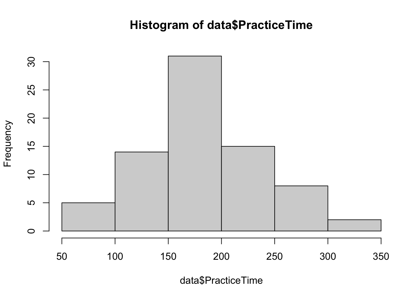
Off to SPSS—click the .sav file and open in SPSS. Reference the following instructions to complete the same tasks.