10 Inferential Statistics (10/3-10/5)
Today we will …
Identify and evaluate dependent and independent group designs
Review connection between experimental designs and threats to study validity
Analyze data using dependent and independent samples t-tests
So we can …
- Acquire an operational understanding of hypothesis testing as it relates to experimental design
I’ll know I have it when …
- I can identify the appropriate statistical test for a research context/research question
Warm up question: Can you identify some phenomenon, test, or other measurable thing that is different for two groups of people? Three groups of people? What might explain those differences?
10.1 The Role of Statistics in Hypothesis Testing
A hypothesis is a proposed solution to a problem. Hypothesis testing is a means to take a rational (logical) decision based on observed data. Statistical tests are designed to reject or fail to reject a null hypothesis based on data. They do not allow you to find evidence for the alternative; just evidence for/against the null hypothesis. Assuming that \(H_0\) is true, the p-value for a test is the probability of observing data as extreme or more extreme than what you actually observed (i.e., how surprised should I be about this?).
The significance level \(\alpha\) is what you decide this probability should be (i.e., the surprise threshold that you will allow), that is, the probability of a Type I error (rejecting \(H_0\) when it is true). Oftentimes, \(\alpha = 5\% = 0.05\) is accepted although much lower alpha values are common in some research communities, and higher values are used for exploratory research in less defined fields. If we set \(\alpha = 0.05\), we reject \(H_0\) if p-value < 0.05 and say that we have found evidence against \(H_0\).
Note that statistical tests and methods usually have assumptions about the data and the model. The accuracy of the analysis and the conclusions derived from an analysis depend on the validity of these assumptions. So, it is important to know what those assumptions are and to determine whether they hold.
10.2 Tests of Group Differences
Before testing whether means are different among groups, it can be helpful to visualize the data distribution.
library(tidyverse)
data(mtcars)
ggplot(mtcars) +
geom_boxplot(aes(x = am, y = mpg, group = am)) 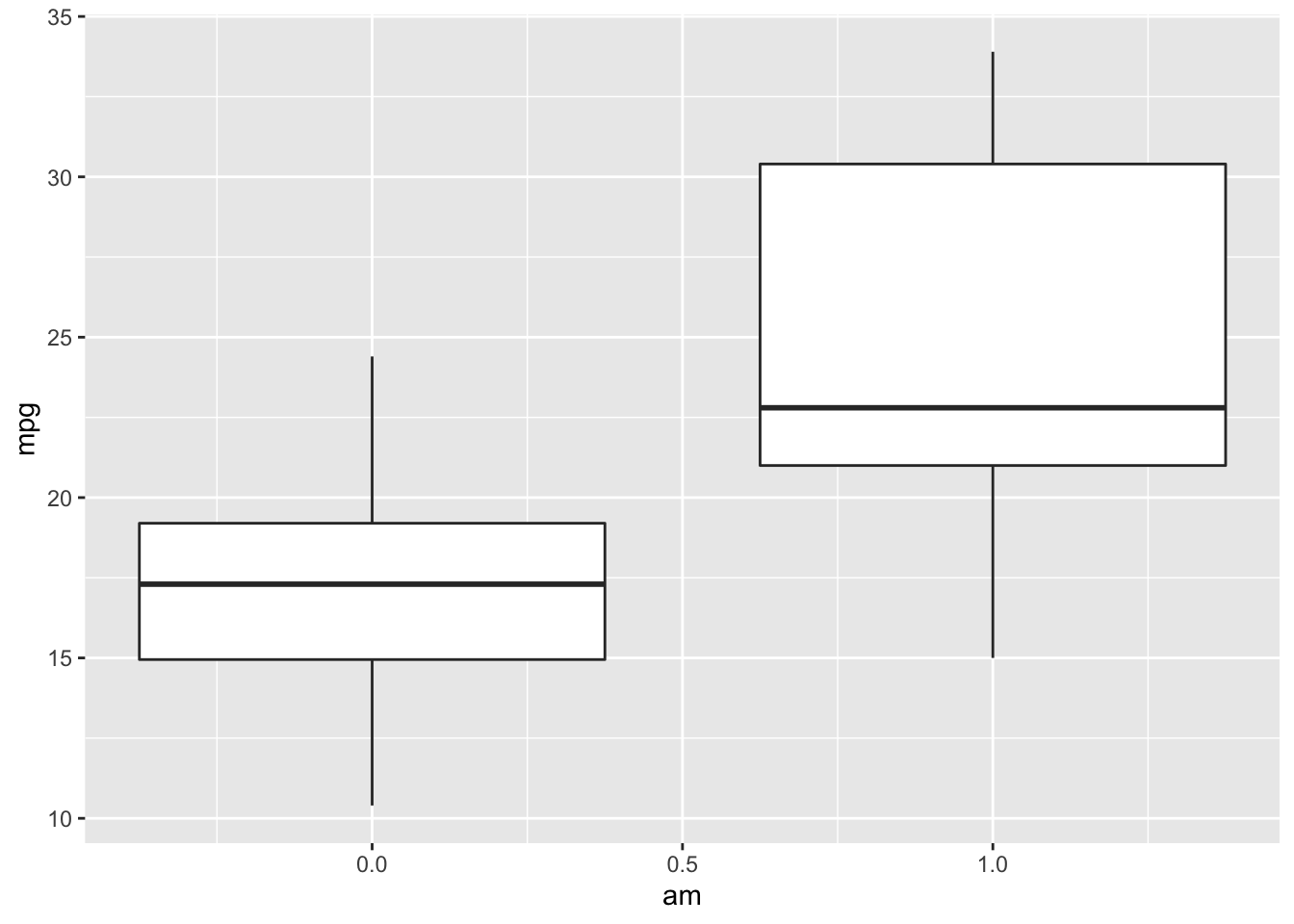
Violin plots are similar to box plots except that violin plots show the probability density of the data at different values.
ggplot(mtcars) +
  geom_violin(aes(x = am, y = mpg, group = am))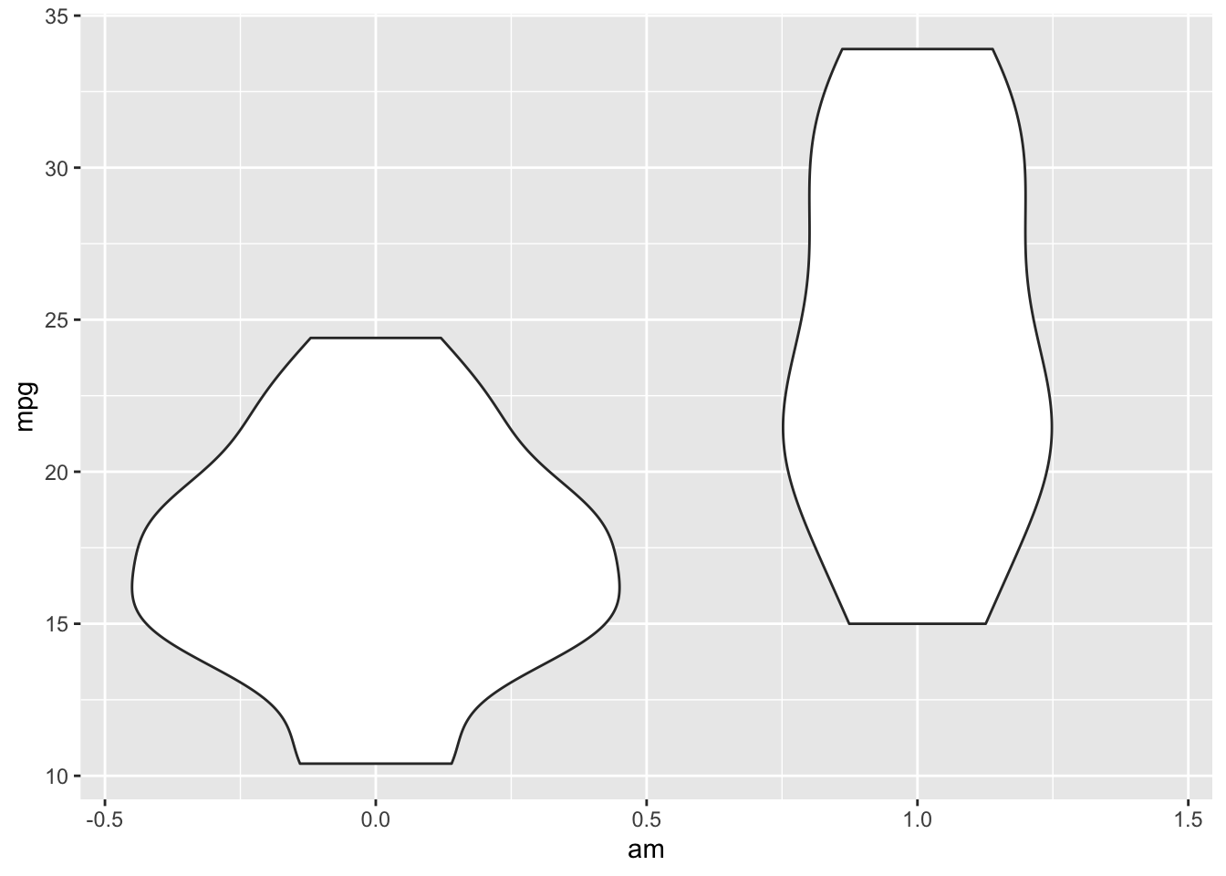
T-tests can be used to test whether the means of two groups are significantly different. The null hypothesis \(H_0\) assumes that the true difference in means \(\mu_d\) is equal to zero. The alternative hypothesis can be that \(\mu_d \neq 0\), \(\mu_d >0\), or \(\mu_d<0\). By default, the alternative hypothesis is that \(\mu_d \neq 0\).
View(mtcars)
t.test(mtcars$mpg ~ mtcars$am, alternative="two.sided")
##
## Welch Two Sample t-test
##
## data: mtcars$mpg by mtcars$am
## t = -3.7671, df = 18.332, p-value = 0.001374
## alternative hypothesis: true difference in means between group 0 and group 1 is not equal to 0
## 95 percent confidence interval:
## -11.280194 -3.209684
## sample estimates:
## mean in group 0 mean in group 1
## 17.14737 24.39231#install.packages('webr')
library(webr)
model <- t.test(mtcars$mpg ~ mtcars$am, alternative = "two.sided")
plot(model)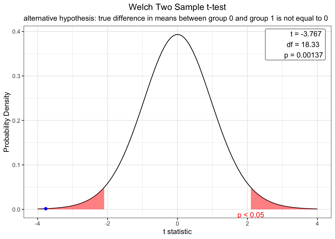
The t -est results indicate that there is a significant difference in mpg between cars with a manual (0) and automatic (1) transmission (t = -3.77, p < .01). The webr library also allows you to easily produce distribution plots. Using this plot, we can determine that the null hypothesis will only be true (no difference between mpg by transmission type) < .01% of the time. Most differences are significant (p < .05) when t values exceed +- 1.96. As such, we can conclude that data from a distribution of mpg for automatic transmissions will only be similar to those of manual transmissions around 1% of the time.
T-tests require a normality assumption which may or may not be valid depending on the situation. The function wilcox.test allows us compare group medians (not means) in a non-parametric setting (i.e., without the assumption of the data coming from some probability distribution). You may have heard of the Mann-Whitney U test. This test is just a two-sample Wilcoxon test. Is the median mpg different for automatic and manual cars?
wilcox.test(mtcars$mpg ~ mtcars$am)##
## Wilcoxon rank sum test with continuity correction
##
## data: mtcars$mpg by mtcars$am
## W = 42, p-value = 0.001871
## alternative hypothesis: true location shift is not equal to 0Yes, there is a significant difference in the median of mpg across transmission types (W = 42, p = .002)
10.2.1 Glossary of Inferential Statistics
Standard Error of the Mean: Standard error is calculated by dividing the standard deviation of the sample by the square root of the sample size. These are represented as
t-values: or the ratio of the departure of the estimated value of a parameter from its hypothesized value to its standard error.
W values: are derived from the non-parametric Wilcoxon test and represent the sum of the ranks in one of both groups.
p-values: represent the statistical significance of a difference in relation to level of accepted error (alpha value)
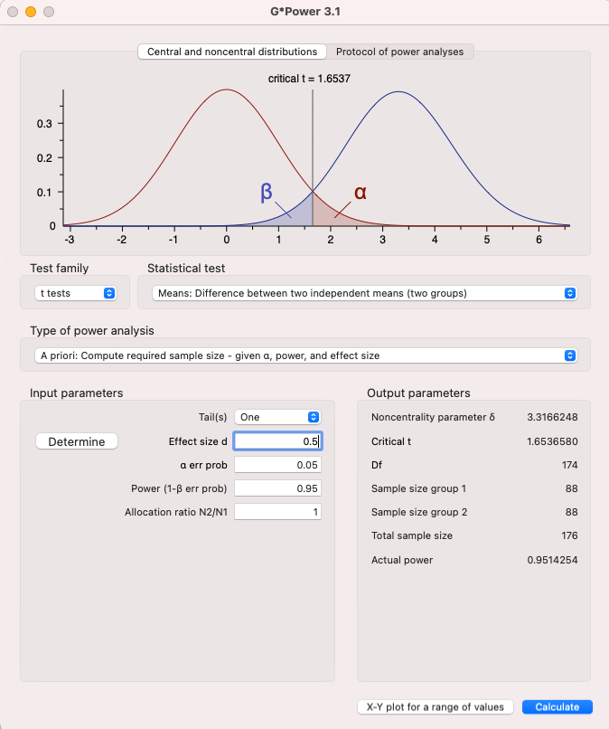
Cohen’s d: Refers to effect sizes as small (d = 0.2), medium (d = 0.5), and large (d = 0.8) based on benchmarks suggested by Cohen (1988). A Cohen’s d of 1 indicates that the means of the two groups differ by 1.000 pooled standard deviation (or one z-score). A pooled standard deviation is a weighted (by sample size) average of the standard deviation (variances) from two or more groups of data when they are assumed to come from populations with a common standard deviation.
Degrees of freedom: the sample size minus the number of parameters you intend to estimate. Represents the maximum number of logically independent values, which are values that have the freedom to vary, in the data sample.
Levenes Test: Test used for the t-test assumption, homogeneity of variance.
F-values: are like t values, but with models that have more than two groups or factor levels.
Tukey’s HSD (honestly significant difference) test: used to determine whether means are different from each other in ANOVA models.
10.2.2 Inferential Modeling
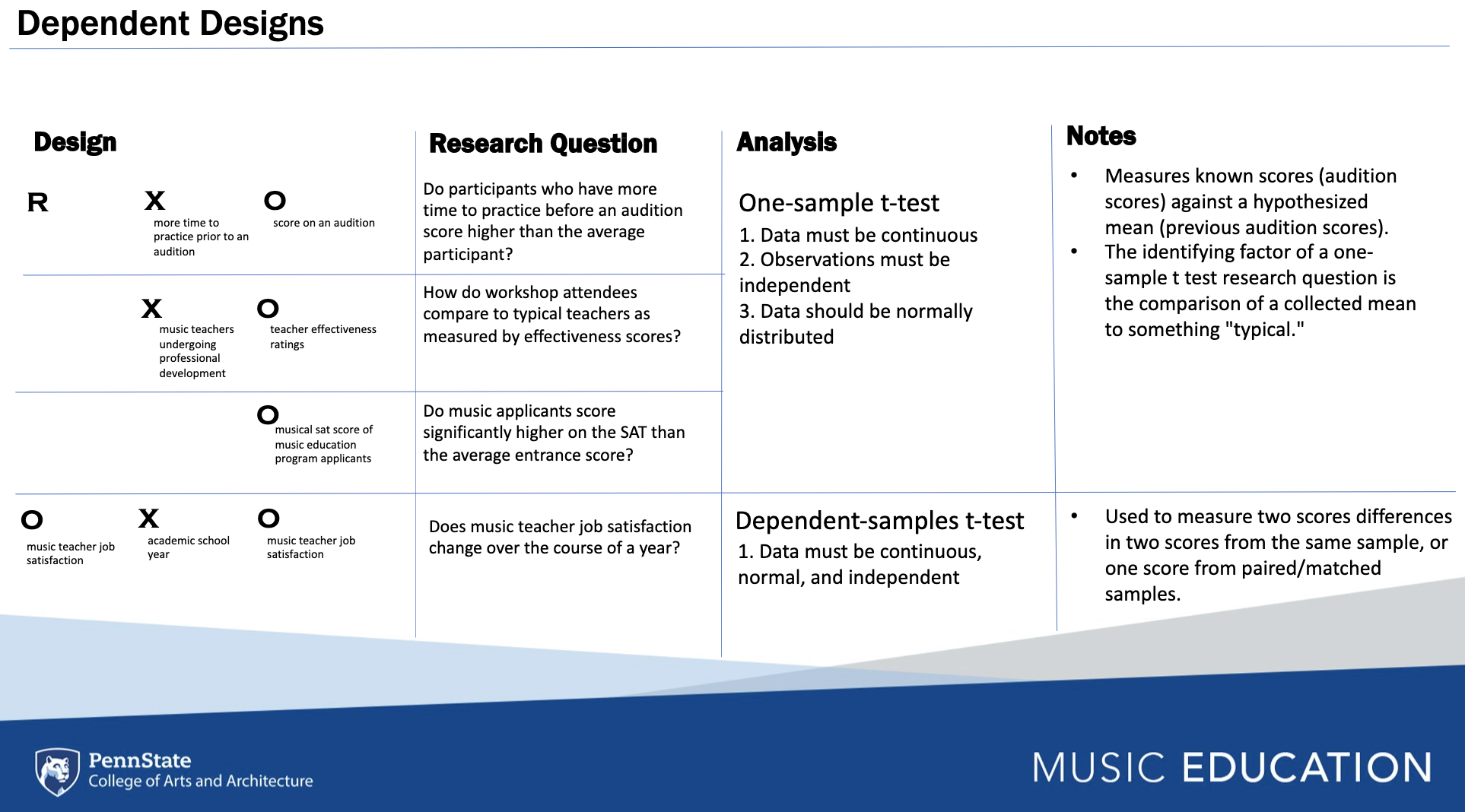
In this section, each chunk will include the code for running an univariate method of statistical analysis in baseR and other libraries. The figure below describes four separate dependent designs that are associated with two basic inferential models which can be analyzed using a one-sample t-test, where a mean with an unknown distribution (e.g., M = 48) is assessed against a known distribution of data. The dependent samples t-test is used to measure score differences from paired or matched samples.
10.2.2.1 One Sample T-Test
We’re going to use the band participation dataset for these examples.
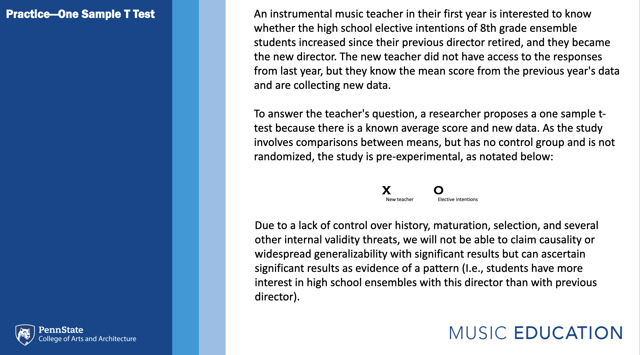
For the one sample t-test, call in the vector where your data are loaded from, and use the argument mu to define the previously known mean (with an unknown distribution). Examine both the output of the statistical test and the automated written report.
data <- read_csv('participationdata.csv')

t.test(data$intentionscomp, mu = 5)
##
## One Sample t-test
##
## data: data$intentionscomp
## t = 9.6215, df = 41, p-value = 4.497e-12
## alternative hypothesis: true mean is not equal to 5
## 95 percent confidence interval:
## 11.17032 14.44873
## sample estimates:
## mean of x
## 12.80952library(report)
onesamplewriteup <- t.test(data$intentionscomp, mu = 5)
report(onesamplewriteup)## Effect sizes were labelled following Cohen's (1988) recommendations.
##
## The One Sample t-test testing the difference between data$intentionscomp (mean
## = 12.81) and mu = 5 suggests that the effect is positive, statistically
## significant, and large (difference = 7.81, 95% CI [11.17, 14.45], t(41) = 9.62,
## p < .001; Cohen's d = 1.48, 95% CI [1.04, 1.92])10.2.2.2 Dependent Sample T-Test
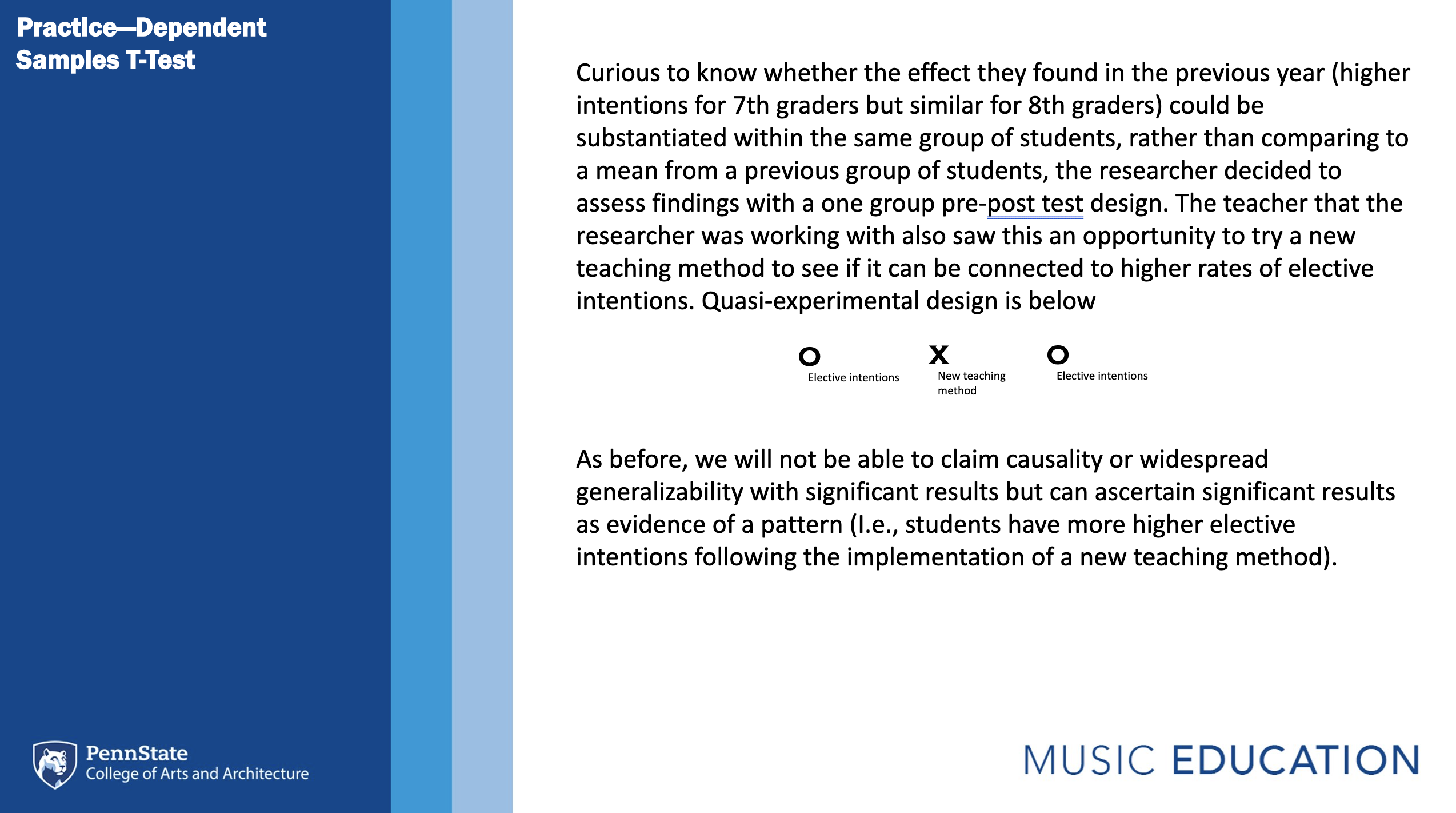
To run a dependent sample t-test, use the function t.test with the argument paired = TRUE
t.test(data$Intentions1, data$Intentions2, paired = TRUE)##
## Paired t-test
##
## data: data$Intentions1 and data$Intentions2
## t = 0.13838, df = 41, p-value = 0.8906
## alternative hypothesis: true mean difference is not equal to 0
## 95 percent confidence interval:
## -0.3236625 0.3712815
## sample estimates:
## mean difference
## 0.02380952dependentsamplewriteup <- t.test(data$Intentions1, data$Intentions2, paired = TRUE)
report(dependentsamplewriteup)## Effect sizes were labelled following Cohen's (1988) recommendations.
##
## The Paired t-test testing the difference between data$Intentions1 and
## data$Intentions2 (mean difference = 0.02) suggests that the effect is positive,
## statistically not significant, and very small (difference = 0.02, 95% CI
## [-0.32, 0.37], t(41) = 0.14, p = 0.891; Cohen's d = 0.02, 95% CI [-0.28, 0.32])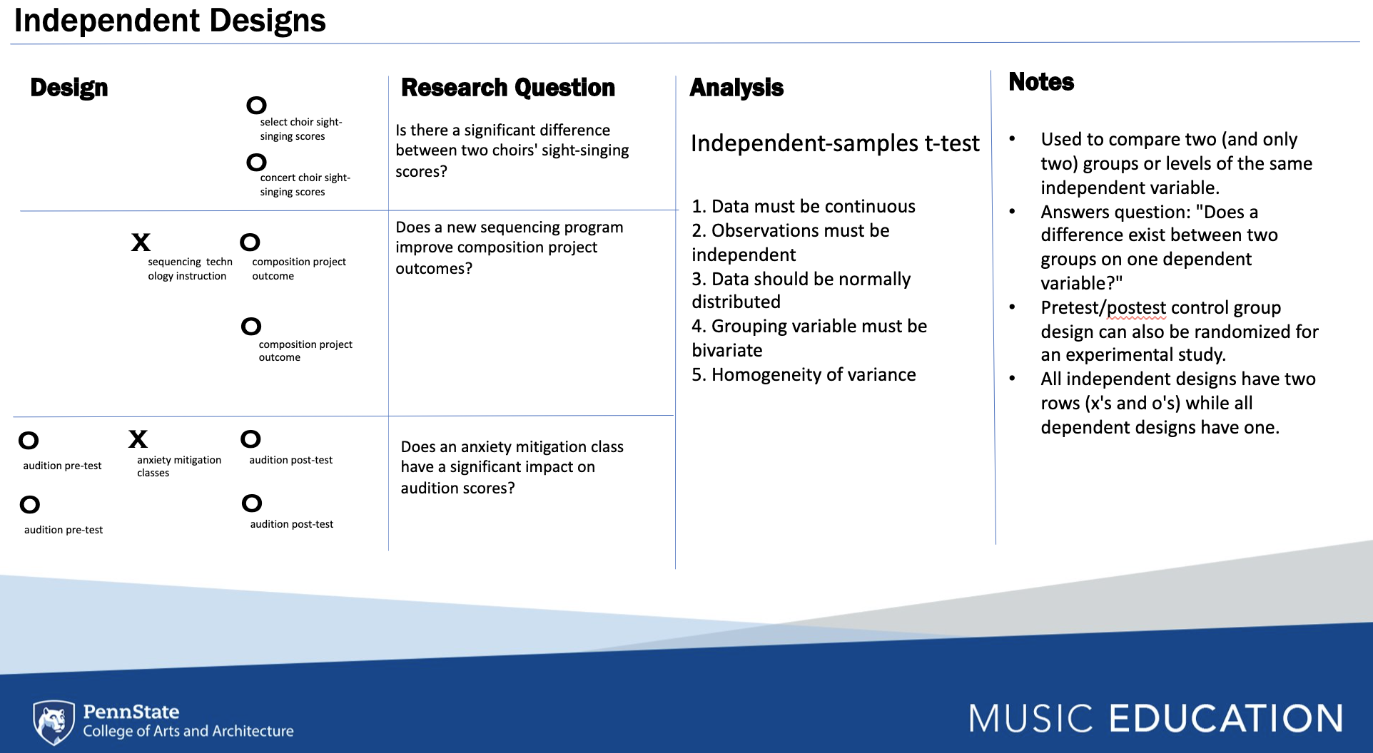
Independent designs are used to compare a measures across differing samples, whereas dependent designs assess differences within a sample.
10.2.2.3 Independent Samples T-Test
Here is another chance to run a t-test
#install.packages('car')
library(car)
## Loading required package: carData##
## Attaching package: 'car'## The following object is masked from 'package:psych':
##
## logit## The following object is masked from 'package:dplyr':
##
## recode## The following object is masked from 'package:purrr':
##
## somelibrary(psych)
leveneTest(data$intentionscomp ~ data$GradeLevel)## Warning in leveneTest.default(y = y, group = group, ...): group coerced to
## factor.## Levene's Test for Homogeneity of Variance (center = median)
## Df F value Pr(>F)
## group 1 0.2425 0.6253
## 38psych::describe(data$intentionscomp)## vars n mean sd median trimmed mad min max range skew kurtosis se
## X1 1 42 12.81 5.26 15 13.24 4.45 3 18 15 -0.52 -1.36 0.81shapiro.test(data$intentionscomp)##
## Shapiro-Wilk normality test
##
## data: data$intentionscomp
## W = 0.83499, p-value = 2.701e-05t.test(data$intentionscomp ~ data$GradeLevel, var.equal = T)##
## Two Sample t-test
##
## data: data$intentionscomp by data$GradeLevel
## t = -2.9009, df = 38, p-value = 0.006156
## alternative hypothesis: true difference in means between group eighth-grade and group seventh-grade is not equal to 0
## 95 percent confidence interval:
## -8.125373 -1.446055
## sample estimates:
## mean in group eighth-grade mean in group seventh-grade
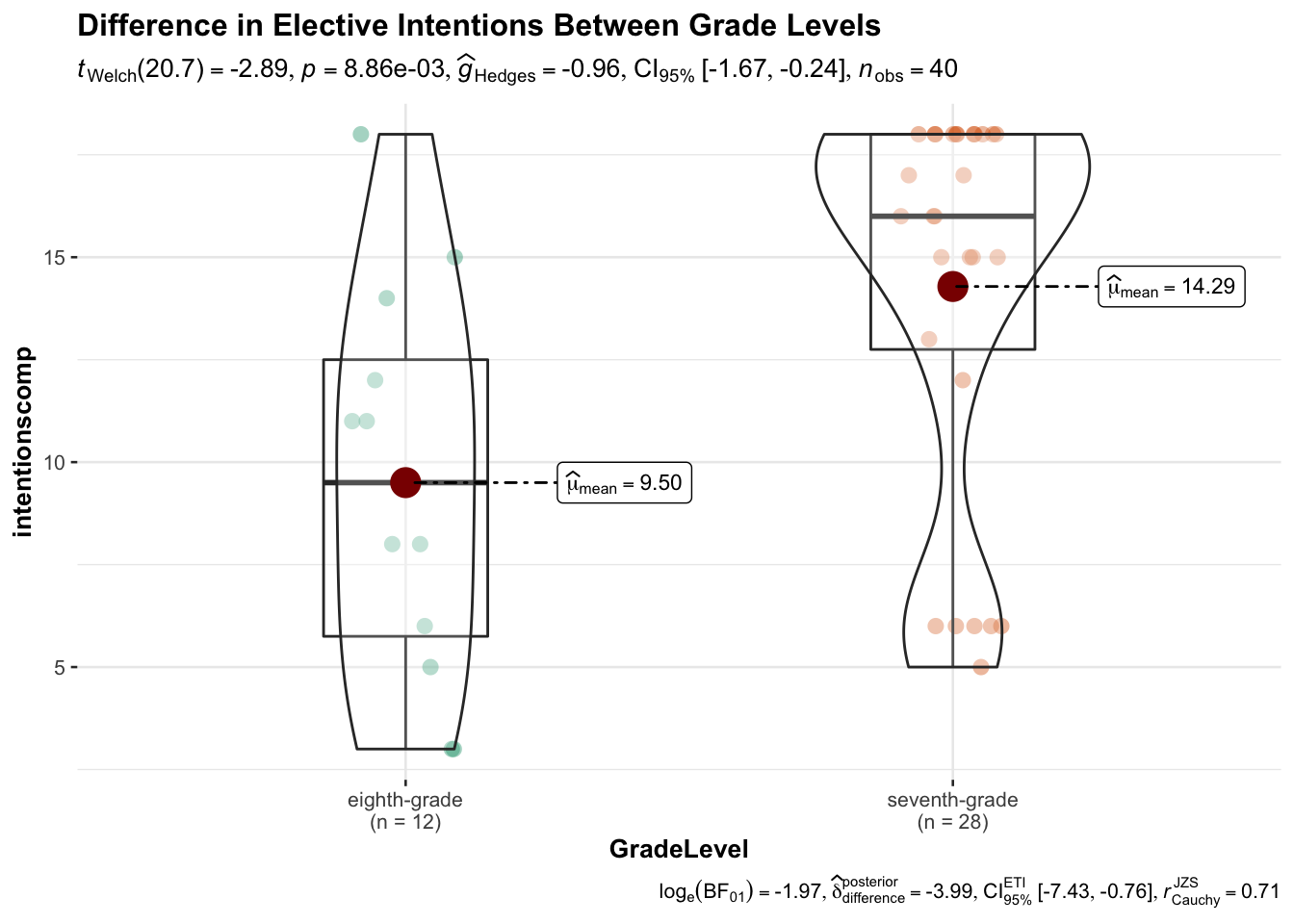
## 9.50000 14.28571Let’s try plotting the difference using ggstatsplot.
library(ggstatsplot)

ggbetweenstats(
  data = data,
  x = GradeLevel,
  y = intentionscomp,
  title = "Difference in Elective Intentions Between Grade Levels"
)
And for the write up?
ttestwriteup <- t.test(data$intentionscomp ~ data$GradeLevel, var.equal = T)
report(ttestwriteup)
## Effect sizes were labelled following Cohen's (1988) recommendations.
##
## The Two Sample t-test testing the difference of data$intentionscomp by
## data$GradeLevel (mean in group eighth-grade = 9.50, mean in group seventh-grade
## = 14.29) suggests that the effect is negative, statistically significant, and
## large (difference = -4.79, 95% CI [-8.13, -1.45], t(38) = -2.90, p = 0.006;
## Cohen's d = -1.00, 95% CI [-1.71, -0.28])10.2.2.4 One-Way ANOVA
There are multiple new terms that emerge when discussing ANOVA approaches. These include:
Within-subjects factors: the task(s) all participants did (i.e., repeated measures)
Between-subjects factors: separate groups did certain conditions (e.g., levels of an experimental variable)
Mixed design: differences were assessed for variables by participants (within-subjects), and something separates them into groups (e.g., between-subjects)
A main effect is the overall effect of a variable on particular groups.
Sometimes you have more than one IV, so you might have two main effects: one for Variable 1 and one for Variable 2.
Also, you can have an interaction between the variables such that performance in “cells” of data is affected variably by the other variable. You can report a significant p-value for the interaction line IF there is a significant main effect p-value.
You can only report a significant interaction if there is a significant main effect.
Interpreting the main effect doesn’t make sense: interpreting the interaction DOES (e.g., the main effect changes based on membership in one of the groups)
One-way ANOVAs are like t-tests, but they compare differences across more than two groups (i.e., categorical variables. For instance, in the participation dataset, you might compare socioeconomic status across the four schools contributing students to the sample. To run the ANOVA, first assign the model using the function aov() with the continuous comparison variable (e.g., SES and the categorical vector of comparison (e.g., School). To see the statistical output, run the summary() function with the model name inside the parenthesis.
model <- aov(SESComp ~ data$School, data = data)
summary(model)
## Df Sum Sq Mean Sq F value Pr(>F)
## data$School 3 2.761 0.9203 8.103 0.000298 ***
## Residuals 36 4.089 0.1136
## ---
## Signif. codes: 0 '***' 0.001 '**' 0.01 '*' 0.05 '.' 0.1 ' ' 1
## 2 observations deleted due to missingnessThe output reflected a significant difference is present among the four schools. However, it is not possible to determine which schools are significantly different from others without Tukey’s HSD, which allows you to examine mean differences between each combination of school. Note the school relationships with a p value below .05 to see what schools differ statistically.
TukeyHSD(model)## Tukey multiple comparisons of means
## 95% family-wise confidence level
##
## Fit: aov(formula = SESComp ~ data$School, data = data)
##
## $`data$School`
## diff lwr upr p adj
## School2-School1 0.6495833 0.2698865 1.02928017 0.0002787
## School3-School1 0.2377315 -0.2033067 0.67876964 0.4764667
## School4-School1 0.3895833 -0.2248980 1.00406464 0.3347392
## School3-School2 -0.4118519 -0.7761699 -0.04753379 0.0215522
## School4-School2 -0.2600000 -0.8219611 0.30196109 0.6023244
## School4-School3 0.1518519 -0.4532475 0.75695122 0.9055435The reporting function produces information regarding the main effect in the model. For more on how to report Tukey’s HSD, visit https://statistics.laerd.com/spss-tutorials/one-way-anova-using-spss-statistics-2.php
report(model)## Warning: Using `$` in model formulas can produce unexpected results. Specify your
## model using the `data` argument instead.
## Try: SESComp ~ School, data =
## data## The ANOVA (formula: SESComp ~ data$School) suggests that:
##
## - The main effect of data$School is statistically significant and large (F(3,
## 36) = 8.10, p < .001; Eta2 = 0.40, 95% CI [0.17, 1.00])
##
## Effect sizes were labelled following Field's (2013) recommendations.Factorial/Two-Way ANOVA
For factorial ANOVAs, there should be more than one categorical independent variable with one dependent variable (more dependent variables should be MANOVA) You are assessing first for main effects (between groups) and then for interaction effects (within groups)
Factorial ANOVAs are named more specifically for their number groupings Some examples are listed below:
2 x 2 x 2 ANOVA = Three independent variables with two levels each (e.g., gender, certified to teach or not, instrumentalist or not—main effects and interaction effects)
2 x 3 x 4 ANOVA = three independent variables, one has two levels (certified or not), one has three levels (teach in a rural, suburban, or urban school) and one has four levels (no music ed degree, music ed bachelors, music ed masters, music ed doctorate)
2 x 3 = two independent variables each one with two levels (gender) another with three levels (degree type)
To conduct a factorial ANOVA in R, use an asterisk to connect the two categorical variables of interest, as seen below. Then, use the summary function, Tukey HSD, and report function to interpret the output.
factorial <- aov(intentionscomp ~ Class*GradeLevel, data = data)
summary(factorial)
## Df Sum Sq Mean Sq F value Pr(>F)
## Class 1 16.6 16.55 0.701 0.40783
## GradeLevel 1 178.1 178.14 7.548 0.00932 **
## Class:GradeLevel 1 16.8 16.82 0.713 0.40415
## Residuals 36 849.6 23.60
## ---
## Signif. codes: 0 '***' 0.001 '**' 0.01 '*' 0.05 '.' 0.1 ' ' 1
## 2 observations deleted due to missingnessTukeyHSD(factorial)## Tukey multiple comparisons of means
## 95% family-wise confidence level
##
## Fit: aov(formula = intentionscomp ~ Class * GradeLevel, data = data)
##
## $Class
## diff lwr upr p adj
## orchestra-band 1.288221 -1.831278 4.40772 0.4078281
##
## $GradeLevel
## diff lwr upr p adj
## seventh-grade-eighth-grade 4.525003 1.125608 7.924398 0.0105076
##
## $`Class:GradeLevel`
## diff lwr upr
## orchestra:eighth-grade-band:eighth-grade 2.6250000 -5.38701652 10.637017
## band:seventh-grade-band:eighth-grade 5.8365385 -0.04267434 11.715751
## orchestra:seventh-grade-band:eighth-grade 5.5083333 -0.21962035 11.236287
## band:seventh-grade-orchestra:eighth-grade 3.2115385 -4.26927785 10.692355
## orchestra:seventh-grade-orchestra:eighth-grade 2.8833333 -4.47920176 10.245868
## orchestra:seventh-grade-band:seventh-grade -0.3282051 -5.28599268 4.629582
## p adj
## orchestra:eighth-grade-band:eighth-grade 0.8139391
## band:seventh-grade-band:eighth-grade 0.0522852
## orchestra:seventh-grade-band:eighth-grade 0.0631394
## band:seventh-grade-orchestra:eighth-grade 0.6577297
## orchestra:seventh-grade-orchestra:eighth-grade 0.7187103
## orchestra:seventh-grade-band:seventh-grade 0.9979489report(factorial)## The ANOVA (formula: intentionscomp ~ Class * GradeLevel) suggests that:
##
## - The main effect of Class is statistically not significant and small (F(1, 36)
## = 0.70, p = 0.408; Eta2 (partial) = 0.02, 95% CI [0.00, 1.00])
## - The main effect of GradeLevel is statistically significant and large (F(1,
## 36) = 7.55, p = 0.009; Eta2 (partial) = 0.17, 95% CI [0.03, 1.00])
## - The interaction between Class and GradeLevel is statistically not significant
## and small (F(1, 36) = 0.71, p = 0.404; Eta2 (partial) = 0.02, 95% CI [0.00,
## 1.00])
##
## Effect sizes were labelled following Field's (2013) recommendations.The more complex a model is the larger the sample size needs to be. As such, the lack of a significant effect may be due to low study power rather than the lack of the phenomenon of interest.
The MANOVA is an extended technique which determines the effects of independent categorical variables on multiple continuous dependent variables. It is usually used to compare several groups with respect to multiple continuous variables.
10.2.2.5 ANCOVA
The Analysis of Covariance (ANCOVA) is used in examining the differences in the mean values of the dependent variables that are related to the effect of the controlled independent variables while taking into account the influence of the uncontrolled independent variables as covariates. Use an addition operator to add covariates to the model.
ancova_model <- aov(intentionscomp ~ GradeLevel + valuescomp, data = data)
summary(ancova_model, type="III")
## Df Sum Sq Mean Sq F value Pr(>F)
## GradeLevel 1 178.9 178.92 9.73 0.00362 **
## valuescomp 1 208.4 208.37 11.33 0.00186 **
## Residuals 35 643.6 18.39
## ---
## Signif. codes: 0 '***' 0.001 '**' 0.01 '*' 0.05 '.' 0.1 ' ' 1
## 4 observations deleted due to missingnessreport(ancova_model)## The ANOVA (formula: intentionscomp ~ GradeLevel + valuescomp) suggests that:
##
## - The main effect of GradeLevel is statistically significant and large (F(1,
## 35) = 9.73, p = 0.004; Eta2 (partial) = 0.22, 95% CI [0.05, 1.00])
## - The main effect of valuescomp is statistically significant and large (F(1,
## 35) = 11.33, p = 0.002; Eta2 (partial) = 0.24, 95% CI [0.07, 1.00])
##
## Effect sizes were labelled following Field's (2013) recommendations.10.3 Research Design Review
Mix and Match Activity
On the board, draw what you believe to be the notation of the experimental designs that I call out.
Scenarios
Creative Activities in an Elementary General Classroom
An elementary general music teacher wants to know whether teaching activities that emphasize creativity and problem solving will boost students’ attitudes toward general music class. The teacher administers an existing measure of music attitude to all primary grade students, and then proceeds to teach using the creativity-intensive approach for the next two weeks. She then gives the students the music attitude measure once again. In comparing students’ scores, the general music teacher observes that almost every student demonstrated improved attitude, and there was a significant gain in average attitude for the entire group of students. The teacher concludes that music class attitudes can be improved by using creative activities in the classroom.
DESIGN: O X O
STATISTICAL TEST: Dependent samples t-test between pre and posttest data
VALIDITY CONCERNS: History, maturation, testing, instrumentation, interaction of testing and maturation, interaction of testing and the experimental variable, interaction of selection and the experimental variable.
Student Teacher Electronic Mentorship Protocol
A music education professor at a college that must place student teachers a long distance from campus decides to use technology to enhance the mentoring of student teachers. The current group of student teachers is randomly assigned to one of two conditions: electronic mentoring or no mentoring (control group). At the end of the semester, each student teacher receives a composite teaching effectiveness rating (university supervisor and cooperating teacher ratings combined). The mean effectiveness rating of students who received electronic mentoring is significantly higher than the mean effectiveness rating of students in the control group. In the future, all student teachers will be required to participate in the electronic mentoring program.
DESIGN: R X O
R O
STATISTICAL TEST: Independent samples t-test between experimental and control group posttests.
VALIDITY CONCERNS: Testing
The Impact of Singing Activities on Aural-Visual Perception of Fourth Grade Students
A beginning orchestra teacher wants to determine whether elementary students’ aural-visual perception can be developed effectively through the use of singing activities. Students in six, fourth-grade classes constituted the study sample. All students completed a test designed to measure aural-visual perception. Three classes proceeded with their “regular” instruction (traditional notation reading), while the remaining three classes used the experimental approach (students sing in addition to reading notation). After three weeks, all participants completed an alternative form of the aural-visual perception measure. The analysis of scores revealed that students who sang while reading notation demonstrated significantly greater gains in perception ability than students engaged in traditional note reading instruction. All other orchestra directors in the district are encouraged to have students sing!
DESIGN: Pretest Posttest Control Group Design (in-tact groups/cluster random sample)
O X O
O O
STATISTICAL TEST: Independent samples t-test
VALIDITY CONCERNS: Interaction of selection and experimental variable (results might be significant only for the chosen population). Interaction of testing and experimental variable (taking the test may teach the participant how to improve. Hawthorne effect
Impact of Composition Activities on High School Band Retention
A researcher wants to know whether including composition activities in high school band classes improves the retention of ensemble members. The high school band director agrees to include group composition activities in band one day a week (typically Fridays) for three months. At the April concert, the band performs each group composition. The researcher then collects student course registration data for the next school year. Over 85% of students were planning to continue in band. The band director encourages other high school music teachers in the district to include composition activities in ensemble classes.
DESIGN: One shot case study
X O
STATISTICAL TEST: Descriptive statistics—One sample t-test if we can ascertain mean retention rate from previous year.
VALIDITY CONCERNS: External validity is the focus, descriptive stats do not have internal validity concerns.
Final Exercise: Consider how you might adapt your study, or design an entirely new study, that utilizes a pretest-posttest control group design, with or without randomization.