Chapter 9 T-Test
Within R we can perform 3 types of T-tests, namely an independent samples t-test, a one-sample t-test, and a paired t-test. Within this book, we will discuss all three of these t-tests.
9.1 Independent samples t-test
An independent samples t-test is used to see if a continuous variable is significantly different in 2 groups. The conditions to perform an independent t-test is that the variable from both groups should be normally distributed and that the variables are independent.
To explain this, we will look at an example of the systolic blood pressure of smokers and non-smokers. We start by loading the data, in this case, an SPSS file called sbp_qas.
library(foreign)
sysbloodpressure <- read.spss("sbp_qas.sav", to.data.frame = TRUE)
## re-encoding from UTF-8Before we continue, it is important to make a null hypothesis and an alternative hypothesis. This should be done before we look at the data. If we want to know if there is a difference between the systolic blood pressure of smokers and non-smokers, the null hypothesis can be that there is no difference between the systolic blood pressure of smokers and non-smokers. We also make an alternative hypothesis, and in this case, it is: There is a difference between the systolic blood pressure of smokers and non-smokers. After we have performed the t-test, we can either reject or not accept the null hypothesis based on the P-value.
Now we can start working with the data, and we start by looking at the dimension of this data with the dim() function.
dim(sysbloodpressure)## [1] 32 5Here we see that our data consists of 32 rows and 5 columns.
The dimensions don’t tell us a whole lot, so let’s look at which variables we have and what they look like:
head(sysbloodpressure)## pat_id sbp bmi age smk
## 1 1 135 28.76 45 No
## 2 2 122 32.51 41 No
## 3 3 130 31.00 49 No
## 4 4 148 37.68 52 No
## 5 5 146 29.79 54 Yes
## 6 6 129 27.90 47 YesWe see that we have pat_id, sbp, bmi, age, and smk as variables. For this example only sbp (systolic blood pressure) and smk (smoking no/yes) are important. Furthermore, we can also use the summary() function which we saw in the chapter descriptive statistics.
summary(sysbloodpressure)## pat_id sbp bmi age smk
## Min. : 1.00 Min. :120.0 Min. :23.68 Min. :41.00 No :15
## 1st Qu.: 8.75 1st Qu.:134.8 1st Qu.:30.22 1st Qu.:48.00 Yes:17
## Median :16.50 Median :143.0 Median :33.80 Median :53.50
## Mean :16.50 Mean :144.5 Mean :34.41 Mean :53.25
## 3rd Qu.:24.25 3rd Qu.:152.0 3rd Qu.:37.76 3rd Qu.:58.25
## Max. :32.00 Max. :180.0 Max. :46.37 Max. :65.00As output, we see that the average systolic blood pressure is 144.5 and that we have a total of 17 smokers and 15 non-smokers. However, we are not interested in the average systolic blood pressure, we are interested in whether the systolic blood pressure is different for smokers compared to non-smokers.
We can start by looking at the average systolic blood pressure of smokers and non-smokers. We can do this in different ways, but for now, I will use the by() function. The by() function takes as arguments: the data, then the data on which we want to split, and finally a function (see again ?by). In this case, we want to look at the systolic blood pressure from the data called sys_bloodpressure, we want to split on smoking (smk), and finally, we want to have the average systolic blood pressure.
by(sysbloodpressure$sbp, sysbloodpressure$smk, mean)## sysbloodpressure$smk: No
## [1] 140.8
## ------------------------------------------------------------
## sysbloodpressure$smk: Yes
## [1] 147.8235When we did that, we see that the systolic blood pressure of non-smokers is lower than that of smokers. The systolic blood pressure is 140.8 for non-smokers and 147.82 for smokers.
We can also make this difference visual, for example, by using a boxplot which will be further discussed in the visualization chapter.
boxplot(sysbloodpressure$sbp ~ sysbloodpressure$smk,
        main = "Systolic bloodpressure smokers and non-smokers", xlab = "Smoking (no/yes)", ylab = "Systolic bloodpressure")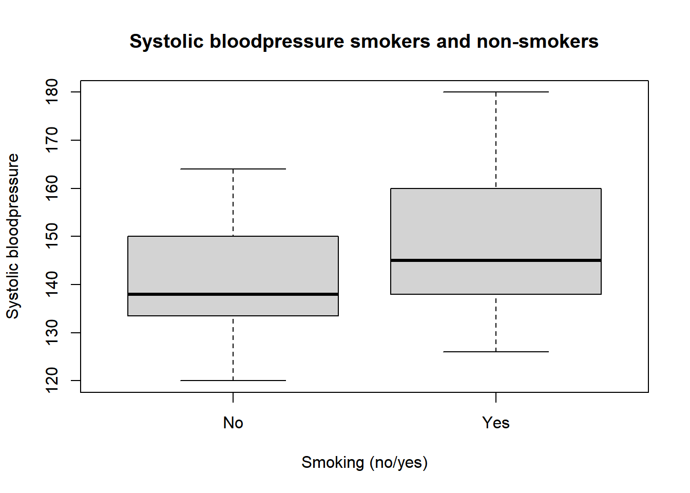
In this boxplot, the Y-axis shows the systolic blood pressure and the X-axis shows whether or not the person is a smoker or a non-smoker. The black line indicates the median of both groups. Therefore, it is not the same as the mean. However, we do see that smokers seem to have a higher (median) systolic blood pressure.
If we want to perform an independent samples T-test, we can use the t.test() function. To do this, we can specify a formula that is similar to what we saw with the by() function. To specify a formula, we use the “tilde” sign and it looks like this: “~”. This sign can often be found under the escape button, but this might be different from one keyboard to another.
To perform the t-test, we first specify for which variable we want to perform the t-test, followed by the ~ sign, and then we specify 2 groups.
t.test(sysbloodpressure$sbp ~ sysbloodpressure$smk)##
## Welch Two Sample t-test
##
## data: sysbloodpressure$sbp by sysbloodpressure$smk
## t = -1.4129, df = 29.963, p-value = 0.168
## alternative hypothesis: true difference in means is not equal to 0
## 95 percent confidence interval:
## -17.17585 3.12879
## sample estimates:
## mean in group No mean in group Yes
## 140.8000 147.8235If we have done that like the example above, we see a lot of things as output. For convenience, we start by looking at the sample estimates. The sample estimates indicate the average systolic blood pressure per group, so in this case, for smokers and non-smokers. Again, we see that these sample estimates are the same as the ones we had when we used the by() function.
Furthermore, we see some important things here. We see the T-statistical (t), how many degrees of freedom there are (df), and the p-value on the second row. We also see the alternative hypothesis: “the real difference in mean systolic blood pressure is not equal to 0”. This alternative hypothesis is quite similar to the alternative hypothesis we made at the beginning of the chapter (there is a difference in the systolic blood pressure of smokers and non-smokers).
Finally, we see the P-value of 0.168. In Health Sciences something is usually seen as statistically significant when the P-value is smaller than 0.05 (Exact sciences might use different p-values for example). In this case, since the P-value is not smaller than 0.05 the conclusion is that we cannot statistically prove that the systolic blood pressure is different for smokers than for non-smokers (we also had a low sample size of only 32 observations). Therefore, we cannot reject the null hypothesis.
9.2 One sample T-test
A One-sample T-test can be used to see if multiple observations deviate from a predetermined mean. For example, if we know that the average grade of the school math exam for the whole country is a 6.6, then we can test if a class that scored on average a 7.4 is statistically different from that mean. Another example is with oatmeal. Suppose we keep track of how many grams of oatmeal there is in our box because we have a feeling that they are not exactly 500 grams, we can test whether the oatmeal boxes we bought are statistically from the 500 grams that was indicated on the box. We will use the oatmeal example in this chapter to explain the one-sample t-test.
Again, we start by making a null hypothesis and an alternative hypothesis:
- Null hypothesis: The boxes of oatmeal we bought are no different than 500 grams.
- Alternative hypothesis: The boxes of oatmeal we bought differ from 500 grams.
Now that we have made the null hypothesis and alternative hypothesis we can move on to the data. For this chapter, we will create our own data. Let’s say that we bought 100 boxes of oatmeal last year and that we weighed all these boxes to see how many grams of oatmeal they contained.
Data generation:
set.seed(100)

oatmeal <- 1:100
grams <- rnorm(n = 100, mean = 495, sd = 3)

oatmeal_data <- data.frame(oatmeal, grams)
As we see above, we created a vector called oatmeal with the numbers 1 to 100 in it to indicate which box of oatmeal it is. Also, we created a vector called grams to keep track of how many grams of oatmeal was in each box. We also see a new function that we haven’t seen before in this book which is the rnorm() function. This function can generate numbers from a normal distribution. This rnorm() function has as arguments: n for how many observations we want, mean for the average of this distribution, and sd for the standard deviation of the normal distribution. In this case, we will obtain 100 numbers from a normal distribution with an average of 490 and a standard deviation of 3. The set.seed() is a new function as well, and this ensures that the results are reproducible. If you were to enter the same code as above with the same seed number, you would get the same numbers back. Afterward, we combine both vectors in a data frame called oatmeal_data. If we look at what the first observations with the head() function we see the following:
head(oatmeal_data)## oatmeal grams
## 1 1 493.4934
## 2 2 495.3946
## 3 3 494.7632
## 4 4 497.6604
## 5 5 495.3509
## 6 6 495.9559Here we see that the first oatmeal box weighs 493.5 grams and the fourth oatmeal box weighs 497.7 grams, and so on.
We can also use the summary() function again.
summary(oatmeal_data)## oatmeal grams
## Min. : 1.00 Min. :488.2
## 1st Qu.: 25.75 1st Qu.:493.2
## Median : 50.50 Median :494.8
## Mean : 50.50 Mean :495.0
## 3rd Qu.: 75.25 3rd Qu.:497.0
## Max. :100.00 Max. :502.7We see that the minimum is 1, and the maximum is 100, and this indicates that we have measured 100 boxes of oatmeal. We can see that the average box of oatmeal weighs 495 grams, the lowest amount of oatmeal was 488.2 grams, and the maximum amount of oatmeal was 502.7 grams.
Now that we have our data of oatmeal boxes, we can test if these 100 boxes of oatmeal are statistically different from the 500 grams. Again, we can do this by using the same t.test() function, but we need to give slightly different arguments.
To perform a one-sample T-test with this data, we can type the following code:
t.test(x = oatmeal_data[["grams"]], alternative = "two.sided", mu = 500)##
## One Sample t-test
##
## data: oatmeal_data[["grams"]]
## t = -16.3, df = 99, p-value < 2.2e-16
## alternative hypothesis: true mean is not equal to 500
## 95 percent confidence interval:
## 494.4011 495.6163
## sample estimates:
## mean of x
## 495.0087Let’s first zoom in on which arguments we need to specify before we look at the output. To perform the one-sample T-test we give an argument for x, and this should be the data you want to test. We also have an argument called “alternative” and this is set to “two.sided”. By default, the alternative argument is set to “two.sided” so you can omit this argument, and the result will be the same. The reason that I did specify it here is because we will look at what other arguments we can specify for this “alternative” argument. We also have an argument called “mu” and here we specify what the average should be. In this case, we specify that boxes of oatmeal should be 500 grams.
Now we will look at the output of the T-test, and we will start by looking at the sample estimates. Here we see the number 495.0087 which indicates that the boxes of oatmeal we measured were on average 495 grams. If we look at the row under data, then we will find the T-statistical (t), the degrees of freedom (df), and the p-value there. Here we see that the P-value is so low that it uses a scientific notation (this is R’s way of dealing with small numbers). 2.2e-16 Is the same as 2.2*10^-16. Since this p-value is far below 0.05, we can reject the null hypothesis and accept the alternative hypothesis that the boxes of oatmeal we bought differ from 500 grams.
We have three options for the alternative argument. The first was “two.sided”. Apart from “two.sided”, we also have “greater”, and “less”. If we specify two.sided, we assume that the observations can differ on both sides of the normal distribution. For example, if we say that the boxes of oatmeal differ from 500 grams, then our observations may be larger or smaller than 500 grams. This is the reason why you should always make a null hypothesis and an alternative hypothesis before you see the data. For example, giving “less” to the alternative argument could be used if the null hypothesis and alternative hypothesis are as follows:
- Zero hypothesis: The boxes of oatmeal do not differ from 500 grams
- Alternative hypothesis: The boxes of oatmeal are on average less than 500 grams.
If you have a predetermined direction, then you can specify “less” (or “greater”), and then the T-test will only test whether the boxes of oatmeal are on average less than 500 grams (or vice versa).
9.3 Paired T-test
Finally, we have the paired t-test and we can use this test when we have 2 measurements from 1 group. This might be the case with repeated measurements such as measuring the weight of persons before and after a diet (2 measurements at different time points). We are going to use this example to explain the paired t-test.
First of all, we need to have data. For this example, we have tracked the weight of 20 people who have been on a diet for two weeks. Since our data is in an excel file, we need the readxl package again.
library(readxl)

diet <- read_excel("diet.xlsx")
Now we have loaded the data and saved it to the diet variable, we can look at the first six observations by using the head() function.
head(diet)## # A tibble: 6 x 3
## id weight_before weight_after
## <dbl> <dbl> <dbl>
## 1 1 65 63
## 2 2 75 73
## 3 3 89 88.7
## 4 4 84 84
## 5 5 63 63.2
## 6 6 102 99Here we see that we have 3 columns: the id that indicates which person it was, and we have two columns with the weight (in kilograms) before and after the diet. If we want to see if the weight after the diet is different than the baseline, we can use the paired T-test. However, first of all, we should make a null hypothesis and an alternative hypothesis;
- Null hypothesis: The weight change of the subjects is equal to 0 kilograms.
- Alternative hypothesis: The weight change of the subjects is different from 0 kilograms. And the null hypothesis and alternative hypothesis indicate that we are going to test two-sided.
If we want to perform a paired T-test, we can use the same t.test() function again. Only now, we give an x and a y argument for the data after and before the diet. Apart from that, we also have to give the paired argument to let R know that we want to perform a paired t-test. The code is as follows:
t.test(x = diet$weight_after, y = diet$weight_before, paired = TRUE, alternative = "two.sided")##
## Paired t-test
##
## data: diet$weight_after and diet$weight_before
## t = -2.9658, df = 19, p-value = 0.00794
## alternative hypothesis: true difference in means is not equal to 0
## 95 percent confidence interval:
## -1.219587 -0.210413
## sample estimates:
## mean of the differences
## -0.715In this case, we have the weight_after as x argument and the weight_before as y argument because we expect that the subjects will lose weight. If we put it this way, the sample estimates will be negative as they should be. In this case, the sample estimates show that the subjects lost 0.715 kilograms on average due to the diet. Furthermore, we also see the t-value, degrees of freedom, and the p-value. The p-value is smaller than 0.05, and this means that we can reject the null hypothesis.
We could also give the weight_before as x argument and the weight_after as y argument, but keep in mind that the t-value, confidence intervals, and sample estimates will become positive instead of negative. This is why you should always check if the sample estimates are correct based on the data and how you should interpret the results.