Chapter 7 Indexing and data frames
Now that we know how to load data and what objects and data structures are, we will look at indexing and discuss data frames more thoroughly.
7.1 Indexing
Indexing is selecting elements from vectors, arrays, lists, and data frames. Sometimes we do not want the entire vector, but only a few numbers from it. We can also use indexing to overwrite objects or numbers. For example, if we have a vector that contains the number 10 when in reality it should contain the number 100 then we can change that by using indexing.
7.1.1 Vectors
Let’s start by looking at how we can index vectors. First, we start by creating a vector and call this variable vector1 for this example.
vector1 <- c(10, 40, 80, 60, 90, 130, 200)
vector1
## [1] 10 40 80 60 90 130 200If we want to select the first element from this vector, then we can use brackets [ ]. To index the number 10 from this vector, we can execute the following code:
vector1[1]## [1] 10First, we start with the name of our variable and then we open a bracket, put in which element we want to get out of our vector and then we close the bracket again.
Similarly, if we want to index the number 80 which is the third element then we put three within the brackets:
vector1[3]## [1] 80We can also index multiple elements by specifying a vector within the brackets.
For example, we can index the 3rd and 4th elements (80 and 60) from the vector by specifying the vector 3:4 within the brackets.
vector1[3:4]## [1] 80 60We could also have created a vector by using the c() function which also works for indexing. For example, if we only want the first and last element of the vector (the numbers 10 and 200), then we can do this:
vector1[c(1, 7)]## [1] 10 200Suppose we want the elements 1 through 5 and element 7 as well, then we can do that by using the c() function again and inside we specify 1:5 followed by a comma and then 7.
vector1[c(1:5, 7)]## [1] 10 40 80 60 90 200We can also apply a negative index with the “-” sign and this will prevent that element from being returned. For example, if we want to replicate the example above where we do not want element 6, we can do it in the following way:
vector1[-6]## [1] 10 40 80 60 90 200and then we see that the result is the same. We can also use the - sign within a vector. For example, if we want all elements except the last 3 we could do it like this:
vector1[-c(5:7)]## [1] 10 40 80 60We can also overwrite certain numbers as mentioned at the beginning of the chapter. For example, if we want to change the number 10 in the first position, then we can do that by indexing and assigning another number. This works as follows:
vector1[1] <- 100
vector1
## [1] 100 40 80 60 90 130 200Here we see that we overwrite the first element of vector1 with the number 100 and look at vector1 again we see that the first element is now 100.
We can also overwrite multiple numbers at the same time. For example, if we want to change the 2nd and 3rd element to 300, then we can do the same:
vector1[2:3] <- 300
vector1
## [1] 100 300 300 60 90 130 200The only difference with the previous example is that we need to index multiple elements.
7.1.2 Matrices
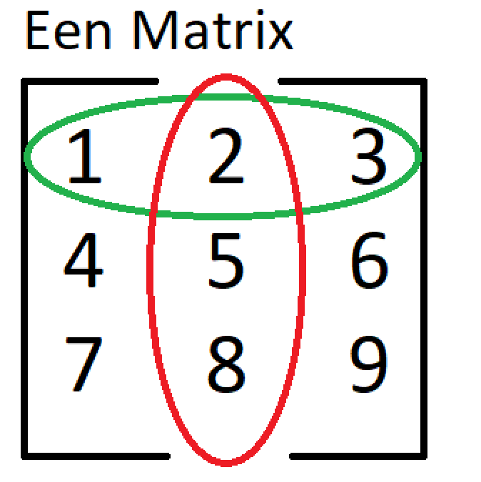
Figure 7.1: Matrix
Before we start indexing matrices it is important to understand the difference between columns and rows. The rows are always horizontal and in the matrix above the first row is encircled in green. Columns are always vertical and in the example matrix, the 2nd column is encircled in red.
Furthermore, it is important to know that R always starts with the rows followed by the columns for indexing purposes.
Now that we know that, we will recreate the example above and save it as example_matrix.
example_matrix <- matrix(1:9, nrow = 3, ncol = 3, byrow = TRUE)
example_matrix
## [,1] [,2] [,3]
## [1,] 1 2 3
## [2,] 4 5 6
## [3,] 7 8 9If we want to get the number 2 from the matrix then we can do that again by indexing. In this example, the number 2 is in the first row and the second column and that means we can get it out as follows:
example_matrix[1, 2]## [1] 2Again we use the brackets [ ] because these are always used for indexing and we specify 1, 2 inside the brackets since this corresponds to the element in the first row and the second column.
We can also do the same for the number 7 which is located in the 3rd row and the 1st column so we will have to put [3, 1] inside the brackets.
example_matrix[3, 1]## [1] 7We can also index complete rows or columns. For example, if we want to have the entire 1st row of the matrix. Then we place 1 inside the bracket to select the first row, and after that, we don’t specify a number for the column.
example_matrix[1, ]## [1] 1 2 3The opposite works as well, for example, if we want to select all numbers from the 2nd column then we omit the number for the row and then after the comma, we specify the number 2 to select the 2nd column only:
example_matrix[, 2]## [1] 2 5 8Finally, we can also perform combinations. Suppose we only want the first two rows from the 3rd column, then we can do that as follows:
example_matrix[1:2, 3]## [1] 3 6In this way, you will get the numbers 3 and 6 as output and not the number 9 from the 3rd column of the matrix.
Again, we can also use the “-” sign to get the same output as the previous example. Here we select the 3rd column and specify that we do not want the 3rd element from that column which is the same as selecting the first and second row from the 3rd column of the matrix.
example_matrix[-3, 3]## [1] 3 67.1.3 Lists
Indexing lists is very similar to indexing vectors with a minor difference. To explain this, we will use the list with students, the grades, and whether they passed or failed which we made earlier in the chapter data types and structures.
names <- c("Sarah", "Hugo", "James")
grades <- c(5, 8, 9)
pass <- c(FALSE, TRUE, TRUE)
class1 <- list(names, grades, pass)
class1
## [[1]]
## [1] "Sarah" "Hugo" "James"
##
## [[2]]
## [1] 5 8 9
##
## [[3]]
## [1] FALSE TRUE TRUEIf we look at the output of this list, then we see that everything is separated with double brackets [[ ]]] with numbers inside. For example, the names are in [[1]], the grades are in [[2]], and whether they passed or not in [[3]]. We also need this information for indexing.
If we want to index the name of our 2nd student we know that it is positioned in [[1]] and on the 2nd position. We can index this name as follows:
class1[[1]][2]## [1] "Hugo"First, we use double brackets [[1]] to select the students, and afterward, we use a single bracket [] to select the element as we did earlier with matrices and vectors.
Furthermore, we can use everything we have learned so far in this chapter. For example, if we only want to know the names of the 2nd and 3rd student we can do it like this:
class1[[1]][2:3]## [1] "Hugo" "James"If we want to know if all students passed or not, then we can use the double brackets only to select that specific part.
class1[[3]]## [1] FALSE TRUE TRUEAs output, we see that 2 students passed and 1 student did not.
7.2 Data frames and indexing data frames
We will now have a closer look at data frames, what kind of functions we can use for data frames, and how we can index data frames.
Throughout this chapter, we will mainly use the iris dataset which we saw briefly in the chapter loading and saving data. Also, you should know that in the “tidyverse” package data frames are referred to as “tibbles”. There are some differences between data frames and tibbles and these differences are beyond the scope of this book.
The iris dataset is automatically available in R, and we can run data(iris) to obtain it.
data(iris)Now we have a variable named iris with the whole dataset.
We can look at this dataset in a kind of excel spreadsheet by using the View() function. If you run View(iris) a new screen will appear and it should be similar to this:
View(iris)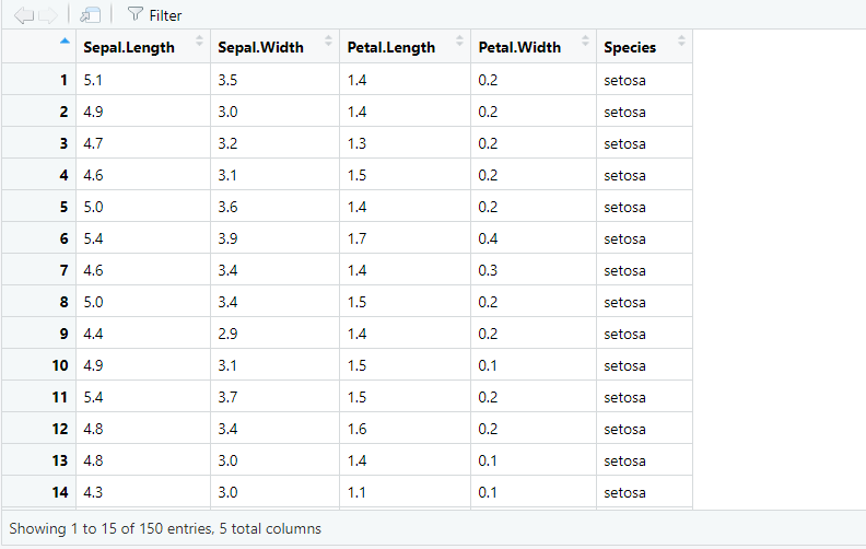
Figure 7.2: Data viewer
At the bottom, it shows how many observations (rows) there are and how many columns there are in total. In this case, we see that there are 150 observations and 5 columns. If the dataset is larger than what will fit on the screen, you can use the arrows in the top right corner to navigate to other columns.
Also, we can obtain the dimensions of the data frame by using the dim() function.
dim(iris)## [1] 150 5As output, we see 150 and 5 and this means that our data frame has 150 rows and 5 columns (remember that the number of rows always comes first).
Furthermore, we can look at the structure of our data frame by using the str() function.
str(iris)## 'data.frame': 150 obs. of 5 variables:
## $ Sepal.Length: num 5.1 4.9 4.7 4.6 5 5.4 4.6 5 4.4 4.9 ...
## $ Sepal.Width : num 3.5 3 3.2 3.1 3.6 3.9 3.4 3.4 2.9 3.1 ...
## $ Petal.Length: num 1.4 1.4 1.3 1.5 1.4 1.7 1.4 1.5 1.4 1.5 ...
## $ Petal.Width : num 0.2 0.2 0.2 0.2 0.2 0.4 0.3 0.2 0.2 0.1 ...
## $ Species : Factor w/ 3 levels "setosa","versicolor",..: 1 1 1 1 1 1 1 1 1 1 ...As output, we see that we have a data frame with 150 observations and 5 variables (columns) and we can see the names of the variables, the first observations, and what data type these variables have. Sepal.Length, Sepal.Width, Petal.Length, and Petal.Width are all numeric data types. Also, we see that Species is a factor data type with 3 levels, namely “setosa”, “versicolor” and “virginica”.
We could also take a look at the first few rows by using the head() function.
head(iris)## Sepal.Length Sepal.Width Petal.Length Petal.Width Species
## 1 5.1 3.5 1.4 0.2 setosa
## 2 4.9 3.0 1.4 0.2 setosa
## 3 4.7 3.2 1.3 0.2 setosa
## 4 4.6 3.1 1.5 0.2 setosa
## 5 5.0 3.6 1.4 0.2 setosa
## 6 5.4 3.9 1.7 0.4 setosaWe can also provide an extra argument to the head() function to display more or fewer rows. By default, it will show the first 6 rows, but you can change this by specifying an extra argument called n = … For example, if we want to see the first 3 rows we can run head(iris, n = 3):
head(iris, n = 3)## Sepal.Length Sepal.Width Petal.Length Petal.Width Species
## 1 5.1 3.5 1.4 0.2 setosa
## 2 4.9 3.0 1.4 0.2 setosa
## 3 4.7 3.2 1.3 0.2 setosaAs output, we now see the first 3 rows instead of the first 6.
Besides the head() function, we also have the tail() function, and this function will show the last few rows. This function is almost identical to the head() function and we can choose how many rows we want to see by proving the n = argument. For example, if we want to see the last 5 rows we can do that as follows:
tail(iris, n = 5)## Sepal.Length Sepal.Width Petal.Length Petal.Width Species
## 146 6.7 3.0 5.2 2.3 virginica
## 147 6.3 2.5 5.0 1.9 virginica
## 148 6.5 3.0 5.2 2.0 virginica
## 149 6.2 3.4 5.4 2.3 virginica
## 150 5.9 3.0 5.1 1.8 virginicaand the output shows the last 5 rows of the iris data frame.
7.2.1 Indexing data frames
We can index data frames in several ways. There are different options to select an entire column. If we want to see all observations of the Sepal.Length column we can run the code iris$Sepal.Length. First, you start with the name of the data frame followed by a dollar sign and then the name of the column you want.
iris$Sepal.Length## [1] 5.1 4.9 4.7 4.6 5.0 5.4 4.6 5.0 4.4 4.9 5.4 4.8 4.8 4.3 5.8 5.7 5.4 5.1
...Normally you will get all observations from the Sepal.Length column as output (in this case 150 observations), but to keep it a bit shorter in the book I will only show the first row as output.
We can also use iris[, “Sepal.Length”] to select the Sepal.Length column and this works similar to indexing matrices. If we leave out the first argument for the rows then R assumes that you want all rows from the Sepal.Length column.
iris[, "Sepal.Length"]## [1] 5.1 4.9 4.7 4.6 5.0 5.4 4.6 5.0 4.4 4.9 5.4 4.8 4.8 4.3 5.8 5.7 5.4 5.1
...We can also use double brackets to select columns in data frames, just as we have seen with lists.
iris[["Sepal.Length"]]## [1] 5.1 4.9 4.7 4.6 5.0 5.4 4.6 5.0 4.4 4.9 5.4 4.8 4.8 4.3 5.8 5.7 5.4 5.1
...One last way is to use single brackets with the name of the column inside:
iris["Sepal.Length"]## Sepal.Length
## 1 5.1
## 2 4.9
## 3 4.7
## 4 4.6
...We can see that this output is slightly different from the others because the observations are now all underneath each other. The reason for this is that if we use single brackets we will get a data frame as output, whereas we get a vector back from the other 3 ways.
So these were 4 ways to select a column from data frames. Personally, I use the dollar sign most often but you can choose whatever way seems easiest to you.
Usually, it’s not very convenient to select a whole column, especially with large datasets since you get all rows back from that particular column. Therefore, you can use another index to select how many rows we want.
For example, if we only want the 5th observation of Petal.Width we can do that as follows:
iris$Petal.Width[5]## [1] 0.2As output, we see that the 5th observation of Petal.Width is 0.2.
We can also select multiple observations by specifying a vector. Suppose we want to see observations 10 to 15 of Petal.Width then we can do that too.
iris$Petal.Width[10:15]## [1] 0.1 0.2 0.2 0.1 0.1 0.2In the 2 examples above I used the dollar sign again, but you can also use the other 3 ways to select columns. For example, if we want to see the first 5 observations of species we can also use single brackets, or double brackets to select the column and then index the first 5 observations.
iris[["Species"]][1:5]## [1] setosa setosa setosa setosa setosa
## Levels: setosa versicolor virginicaWe can also overwrite certain observations with indexing. For example, if we know that the first observation from species shouldn’t be setosa, but virginica instead we can do that as follows:
iris[["Species"]][1] <- "virginica"
iris[["Species"]][1]
## [1] virginica
## Levels: setosa versicolor virginicaAnd now we see that the first observation of Species has changed to virginica.
Finally, we can also add new columns in a data frame. For example, if we have length and weight in a data frame then we can also calculate BMI with those 2 columns.
As an example, we are going to create a new column called Petal_WL and we are going to create this column by multiplying Petal.Length and Petal.Width.First, we start with the name of our dataset iris and then we index a column that does not exist yet. Afterward, we can assign values to this new column by using the <- sign.
iris[["Petal_WL"]] <- iris$Petal.Length * iris[, "Petal.Width"]In the example above I selected the columns in three different ways to show that you can do it with different methods. However, from a practical point of view, it is easier to choose one method and stick with it. The only thing that will not work for this example is using single brackets. If we use iris[“Petal.Width”] it will return a data frame as output and we cannot multiply 2 columns in this way.
After we have run the code we can see that there is no output. However, if we now look at the first 6 rows of the data frame with the head() function:
head(iris)## Sepal.Length Sepal.Width Petal.Length Petal.Width Species Petal_WL
## 1 5.1 3.5 1.4 0.2 virginica 0.28
## 2 4.9 3.0 1.4 0.2 setosa 0.28
## 3 4.7 3.2 1.3 0.2 setosa 0.26
## 4 4.6 3.1 1.5 0.2 setosa 0.30
## 5 5.0 3.6 1.4 0.2 setosa 0.28
## 6 5.4 3.9 1.7 0.4 setosa 0.68then we see that there is a new column in our data frame called Petal_WL. We can also see that this column is the result of multiplying Petal.Length and Petal.Width for each row. For example, we see that the first 2 observations from Petal_WL are 0.28 and that these were obtained by multiplying 1.4 by 0.2.