Chapter 2 Possibilities within the RStudio environment
RStudio is called an integrated development environment (IDE). If you are not a programmer this word will probably not mean anything but in this chapter I will try to explain why it is convenient to use RStudio.
2.1 First steps with R
To see what the difference is between R and RStudio we will first look at what R looks like. If you created a shortcut of R in the previous chapter you will find 2 versions of R on your desktop (a 32-bit version and a 64-bit version).
Figure 2.1: R versions
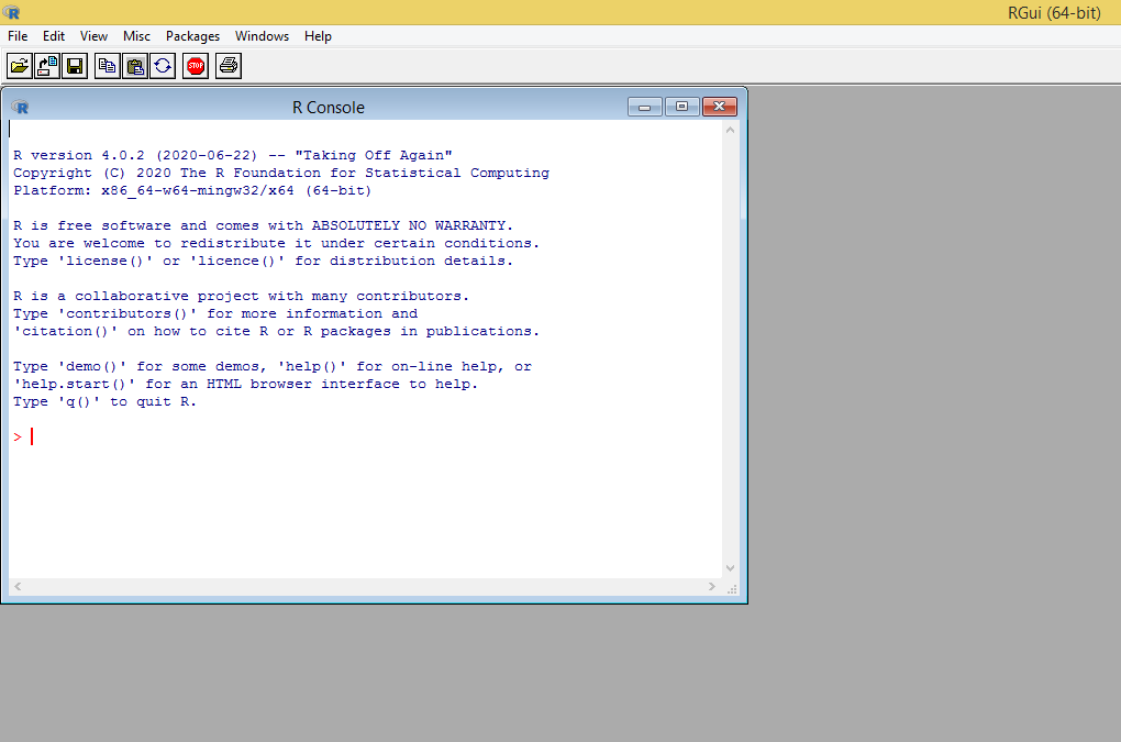
Figure 2.2: Startscreen R
2.2 R as a calculator
In the screen above you can see a red arrow to the right, where you can type all kinds of different things. For example, if you enter 8+12 at the red arrow and then press enter, R will not surprisingly return 20 as output (shown in blue with [1] 20).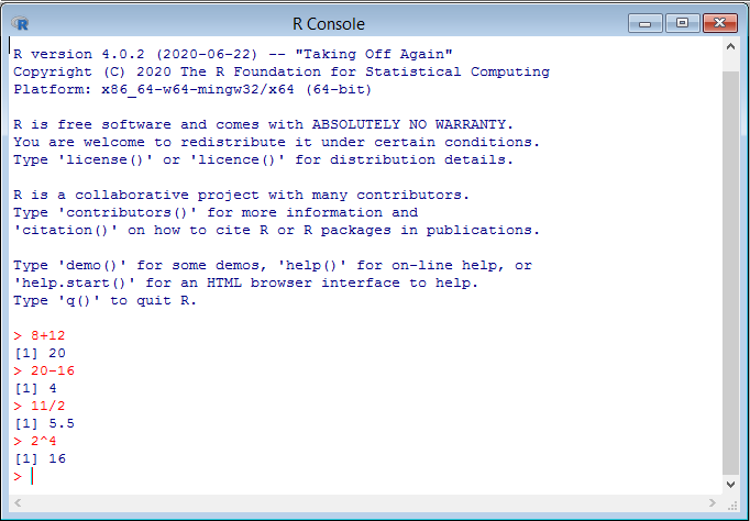
Figure 2.3: Calculator
Besides adding with +, you can also subtract with -, divide with /, multiply with *, and exponentiate with ^. In the example above you also see 2 to the power 4, which is equal to 16.
Furthermore, you have the modulus with two percentages in a row %%. The modulus actually means divide a number by another number, and if something remains, return it as a number. An example of this is 7%%3. 3 Fits 2 times into 7 and then 1 remains which means that the result is 1.
7%%3## [1] 1Another example of the modulus is 6%%3, 3 fits 2 times in 6 and there will be nothing left which means that the result of 6%%3 is 0.
6%%3## [1] 0Finally, we have dividing with rounding down and the sign for this is %/%. For example, if we divide 7 by 3 the result will be 2,333…, but if we type 7%/%3 in R it will round the result to whole numbers, so the result is 2.
7%/%3## [1] 2Furthermore, normal calculation rules apply in R, so this means that multiplication will happen before addition. If we want to calculate 3 + 2 * 5 in R, R will first calculate 2 * 5 and then add 3, so the result of this is 13.
3 + 2 * 5## [1] 13If we want R to first calculate 3 + 2 and then multiply that result by 5 we can use parentheses:
(3 + 2) * 5## [1] 25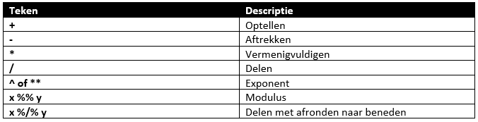
Figure 2.4: Signs
2.3 The assignment operator
Within R you can store certain numbers, and we do this by using the assignment operator which looks like this: <-. It is an arrow to the left and a minus sign on the end.
For example, if we type x <- 10 then R will not return anything as output. But if we then type x it will return the number stored under x.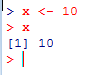
Figure 2.5: Example assignment
We can store multiple numbers under a variable by using vectors (more about vectors will be explained in chapter 8) and we do this by using the c function. For example, if we want to assign multiple numbers to the variable y we use the assignment operator again and use the function c (note: all functions start with a name and are opened and closed with parentheses).
All numbers are separated with a comma and if you type y again in R it will return all numbers stored in the variable y.
y <- c(10, 8, 6, 7, 7.5)
y
## [1] 10.0 8.0 6.0 7.0 7.52.4 Brief introduction to functions
Furthermore, there are a lot of functions we can use with R. For example, you can get the average of multiple numbers by using the mean function. You do this by using the mean() function and within the parenthesis, you place the variable of which you want to get the average. So if we do this for the variable y by typing mean(y) in R after we assigned all numbers to y the result will be 7.7.
mean(y)## [1] 7.72.5 Advantages of RStudio
Now that we have gotten a little familiar with using R as a calculator, the assignment operator, and functions, we will now start using RStudio. To use RStudio you need to have R installed on your computer (so make sure you have gone through the installation chapter). When starting RStudio, the initial screen will be similar to mine: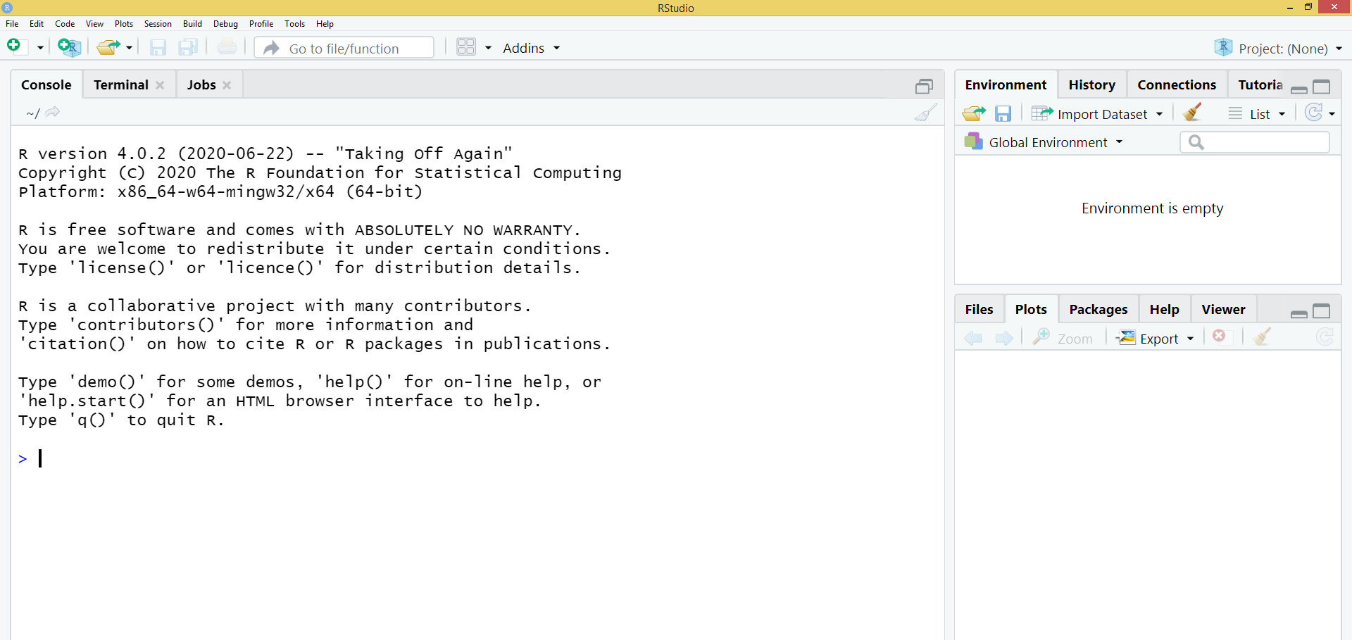
Figure 2.6: Startscreen RStudio
Everything we did at the beginning of the chapter we can also do within RStudio. For example, if we want to calculate something we can do that at the blue arrow. We can also assign numbers to variables and we can use functions again.
2.5.1 The Environment screen
If we type the following in RStudio:
x <- 10
y <- c(1, 2, 3, 4, 5, 6, 7, 8, 9, 10)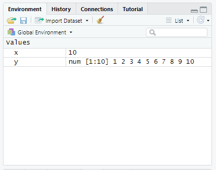
Figure 2.7: Environment screen
The environment screen shows everything that we have loaded or saved within our current R session which provides a quite useful overview.
2.5.2 The Files screen
Below the environment screen, we have the files screen. This screen has a couple of options but is by default on Files.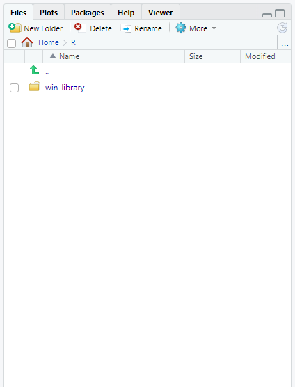
Figure 2.8: Files screen
In this file screen, you can open, delete, or rename certain files.
Next to files we have plots. This screen will automatically open once you made a visualization (more about visualisations in chapter 15). If we take a look at an example image: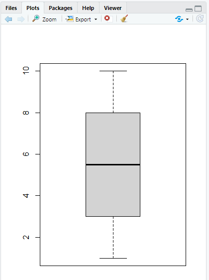
Figure 2.9: Example plot
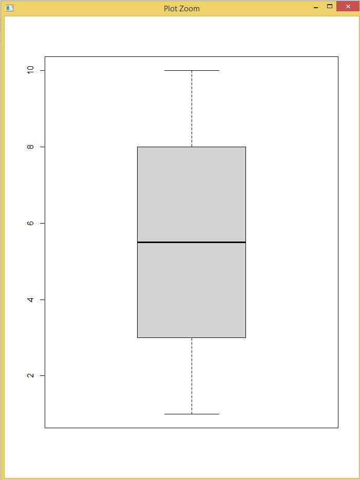
Figure 2.10: Example enlarged plot
With the export button, we can save images on our computer.
In this file screen, we also have the option packages, viewer, and help. The first two are not very important for now, but we are going to look at the help option.
If we click on this help option we will get to the next screen: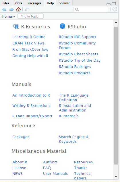
Figure 2.11: Help option
Here are all kinds of helpful links and instructions for R and RStudio.
If we need help for certain functions or we forgot how something works, we can use the ? character. For example, if we no longer know how the average function mean works, we can simply type in RStudio ?mean and the help screen will explain this function: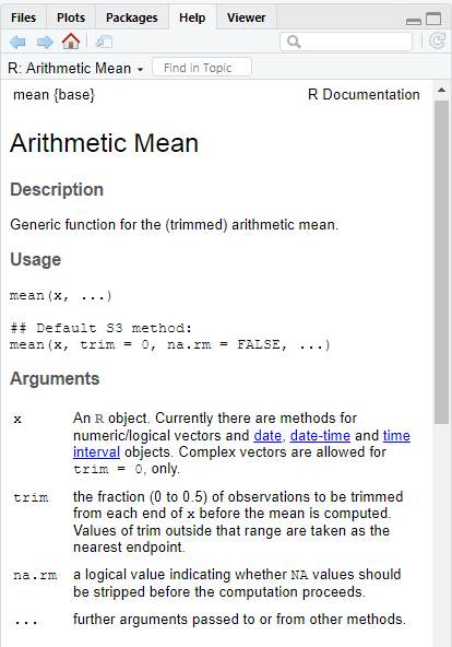
Figure 2.12: Help mean
This will take you to the documentation for the mean function and here you can learn more about the use of the function, what kind of arguments you can give and if you scroll down to the bottom of the screen you will usually find examples under Examples.
I also strongly recommend using google. Almost everything is possible in R and a lot of people use it, so you can find a lot of information on google as well. For example, if we type in google: R how to get mean of a variable. Then there are numerous websites that explain that the mean() function of R can calculate the average of a variable.
2.5.3 The Tab button
Another very useful feature of RStudio is the tab button. For example, if we still know that the average function starts with “me” but don’t know what came after, we can type me in RStudio and then press the tab button. If you do this you will see a scroll menu with all the functions that start with me.
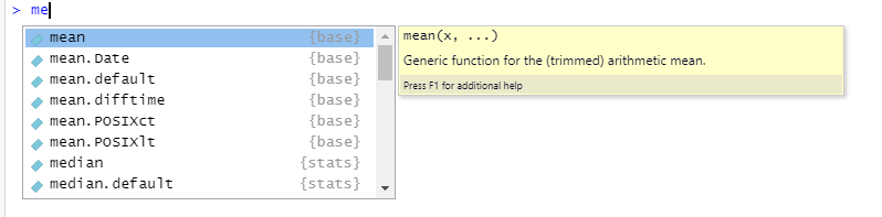
Figure 2.13: Tab button
When you hover your mouse over these functions you will see on the right in yellow a little more about the use of the function and if you click on mean then R will automatically complete me to mean().
2.5.4 Syntax highlighting
Furthermore, we have syntax highlighting in R studio which means that it gives certain things like functions and comments a different color than other things. This makes code more readable. You can also use a different theme, or make the text larger, or choose a different font. You can do this by clicking on Tools > Global options > Appearance at the top of RStudio.
Once you have done that, you will be taken to the next screen:
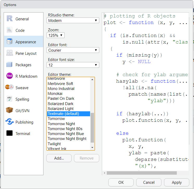
Figure 2.14: Appearance screen
With Editor font size you can choose how big or small you want the text to be and in Editor font size you can choose a different font. You also have Editor theme which is by default set to Textmate. In the right screen, you can see a preview of what it looks like and you can see the syntax highlighting for the default Textmate option. For example, functions are blue, just like certain words like if, else, and NULL. We can choose to set a different theme here, for example, the theme Merbivore.
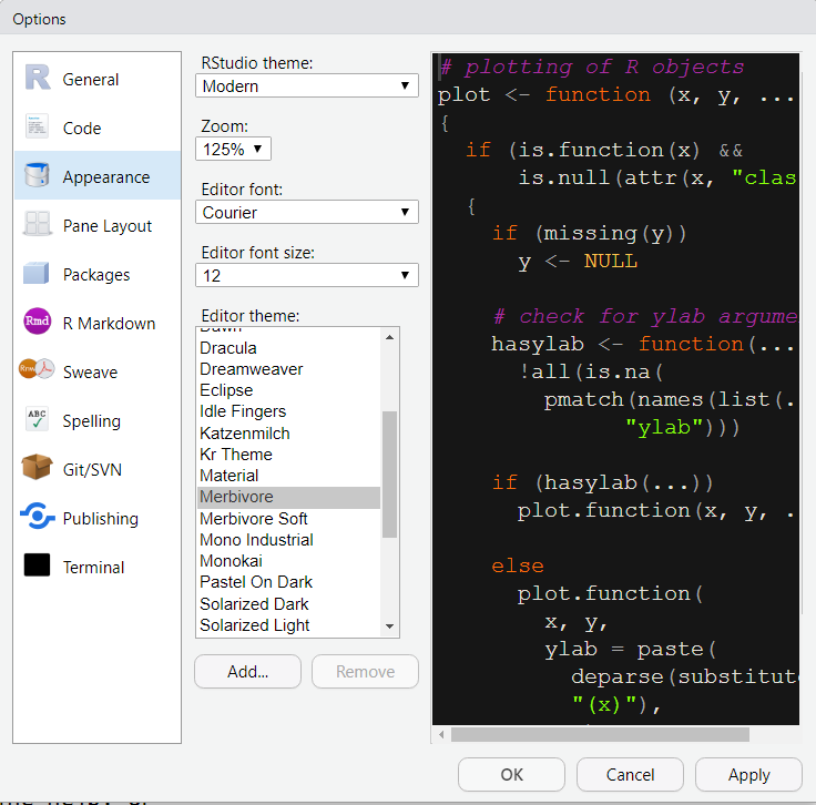
Figure 2.15: Example theme Merbivore
And of course, you could also change it back to other themes by going to Tools > Global options > Appearance in the same way we did before.