Chapter 5 Data types and structures
5.1 Objects
5.1.1 Numeric
First of all, we are going to look at the numeric data type. Numeric is a data type used to store numbers. For example, if we assign the number 6 to a:
a <- 6Then we can look at what kind of data type it is by using the class() function.
class(a)## [1] "numeric"As output, we see that the data type of variable a with the number 6 in it is numeric.
If we assign multiple numbers to a variable b, we see that the outcome of the class function is still numeric.
b <- c(1, 2, 3, 4, 5)
class(b)
## [1] "numeric"Another way to see if something is a numeric data type is to use the is.numeric() function.
is.numeric(a)## [1] TRUEAfter we have used is.numeric() to see if a was a numeric data type we see as output TRUE. This means that a is truly a numeric data type. TRUE is an example of a logical data type and we will look at logical data types later on in this chapter.
In some functions, numeric data types are sometimes referred to as the double data type. This is not important to remember, but if you ever come across the double data type, you should know that they are numeric data types as well.
typeof(a)## [1] "double"5.1.2 Characters
Besides the numeric data type, we also have a character data type. A character data type can be used to store text. An example of a character data type is “hello”.
c <- "hello"
class(c)
## [1] "character"If we assign “hello” to the variable c and then use the class function again the output is “character”. It is important to know that characters are always stored in double parentheses “so this is where the text should be”.
An example of this is when we store numbers as characters.
d <- c("1", "2", "3")
class(d)
## [1] "character"Here we see that if we put numbers inside double parentheses it is not a numeric data type anymore, but it is a character data type now.
5.1.3 Logical
Earlier in this chapter, we mentioned that TRUE was an example of a logical data type. Besides TRUE there is another logical data type and that is FALSE. You will mainly find these logical data types in functions. Functions often have a lot of options or arguments that you may or may not want to perform and you can do that by using TRUE or FALSE. It is important to know that TRUE and FALSE are written in capital letters and if you don’t do that then it will no longer be a logical data type. We can shorten TRUE and FALSE by using T and F respectively.
e <- TRUE
class(e)
## [1] "logical"class(F)## [1] "logical"class(T)## [1] "logical"And not completely surprising we can also test if something is a logical data type by using the is.logical() function just like we did earlier with the is.numeric() and is.character() functions. And the output from this will always be a logical data type; either FALSE or TRUE.
is.logical(TRUE)## [1] TRUEWe may also encounter logical data types in evaluations. For example, if we want to know whether 3 is smaller than 6, we can type the following code:
3 < 6## [1] TRUEThe result of this is TRUE, which indicates that 3 is indeed smaller than 6.
Additionally, we can test whether 10 is larger than 20 by using the right arrow (>) instead of a left arrow (<) to evaluate if one number is larger than the other.
10 > 20## [1] FALSEWe can also check if something is larger or equal to by using the >= sign. For smaller than or equal to we can use the <= sign.
We can also evaluate if a number is exactly the same as the other one by using the == sign.
20 == 20 ## [1] TRUE20 And 20 are exactly the same, and thus R gives TRUE as output. Also, if we assign 20 to variable x and y and then check if x and y are the same we see that this also returns TRUE.
x <- 20
y <- 20

x == y
## [1] TRUEWe also have the != sign, which means that something is not equal to the other number and is the opposite of ==. If we use this again for the example with 20 and 20 then the result is FALSE, since these are equal to each other.
20 != 20## [1] FALSEFinally, we have | and &. The first sign | means: or. For example, if we want to test whether 6 is greater than or equal to 10 or 4, we can type the following code:
6 >= 10 | 4## [1] TRUEThe other character & means: and. If we want to know whether 6 is larger or equal to 10 and 4 we type the following code:
6 >= 10 & 4## [1] FALSENow we see that the result is FALSE because 6 is larger than 4 but not larger than 10.
The result of all these evaluations were all logical data types, namely TRUE of FALSE and we have also seen examples of logical data types.
5.1.4 Factor
The factor data type factor is commonly used in statistical analyses. For example, if we have a dataset with Social Economic Status (SES), it may be coded as “Low”, “Average” and “High”. The only problem is that we can’t use that for statistical analysis because everything has to be coded as numbers if we want to be able to use it for analysis. The factor data type can be used for this. For example, if we have the variable SES with “low”, “average” and “high” and we look at what data type it is, we can see that it is a character because “low”, “average” and “high” are all written in double parentheses.
SES <- c("Low", "Average", "High")
class(SES)
## [1] "character"Now what we can do is change this variable to a factor (Note: We can overwrite variables by assigning something else to the same variable). We can do this by using the as.factor() function.
SES <- as.factor(SES)
class(SES)
## [1] "factor"levels(SES)## [1] "Average" "High" "Low"Now we see thatthe SES variable has become a factor data type. This has assigned numbers or levels to the categories of low, average, and high and in this way, we can use them for statistical analysis. In addition to the as.factor function, we also have several other as. functions and these can change data types to other data types whenever that is possible.
For example, if we have a vector with the numbers 1 to 7 and this is stored as a character data type (in parentheses " "), then we can change it to the numeric data type by using the as.numeric() function.
f <- c("1", "2", "3", "4", "5", "6", "7")
f <- as.numeric(f)
f
## [1] 1 2 3 4 5 6 7class(f)## [1] "numeric"But as mentioned earlier, we can only do that if it is logical, if we try to do it with, for example:
as.numeric("This is an example")## Warning: NAs introduced by coercion## [1] NAThen we see a red error message because R cannot assign values to text.
We can use the as.numeric() function for logical data types as well. Accordingly, TRUE will be encoded as 1 and FALSE will be encoded as 0.
g <- c(TRUE, FALSE, TRUE, TRUE)
as.numeric(g)
## [1] 1 0 1 1Certain functions in R will already do this automatically. For example, if we want to know the sum of the variable g with 3 times TRUE in it and one FALSE in it then R will automatically do this and return the result 3.
sum(g)## [1] 35.2 Structures
There are several important data structures in R. Visually, they look like this:
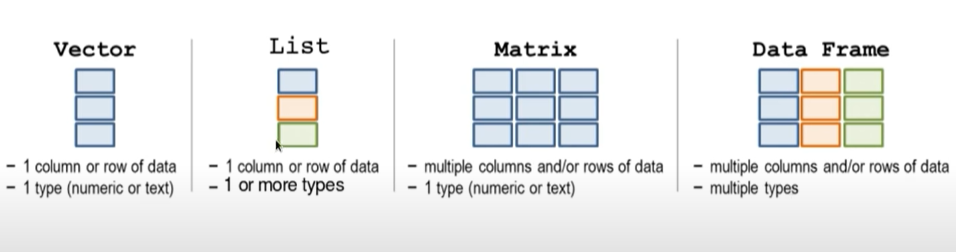
Figure 5.1: Data structures
The difference between these data structures is that vectors and lists can only have one column or row of data. With Matrixes or data frames we are able to store multiple rows or columns of data. Another difference is the amount of data types we can store in these data structures.
5.2.1 Vector
We start by looking at vectors. We have already seen vectors several times before. Vectors are a way to store one type of data in a certain variable. A simple vector we can create is a variable with a number in it. For example, if we assign the number 10 to the variable h and then check if h is a vector with the function is.vector() we will see that the result is TRUE.
h <- (10)
is.vector(h)
## [1] TRUEFurthermore, we have already seen that if we want to store multiple numbers in a vector then we can use the c() function.
i <- c(10, 17, 25, 41)
is.vector(i)
## [1] TRUEFurthermore, we can also create vectors by using the “:” sign. For example, if we want to create a vector with the numbers 1 to 50 (or even more) you can imagine that it will take quite some time if we have to enter them ourselves with the c() function. If we want to do this we can also type the following code:
j <- 1:50
j
## [1] 1 2 3 4 5 6 7 8 9 10 11 12 13 14 15 16 17 18 19 20 21 22 23 24 25
## [26] 26 27 28 29 30 31 32 33 34 35 36 37 38 39 40 41 42 43 44 45 46 47 48 49 50And this is also an example of a vector.
We can also make vectors with only characters. For example, if we want to make a vector with the names of students we can use the c() function again.
k <- c("Peter", "Sarah", "Michiel", "Jimmy")
is.vector(k)
## [1] TRUE5.2.2 List
Lists are very similar to vectors. The only difference between vectors and lists is that we can store multiple data types within lists as opposed to vectors. To illustrate this difference we will take a look at the following example:
l <- c(1, 2, 3, "4")
l
## [1] "1" "2" "3" "4"In this example, we tried to create a vector with the numbers 1 to 3 (numeric data type) and a character “4”. If we look at the output we see that R has also made the numbers 1 to 3 characters. The reason for this is that vectors are only able to store one data type. If we want to store multiple data types in a variable we can use lists.
So if we want to store the numbers 1 to 3 as numeric and the number 4 as a character we can do that by using the list() function to create a list.
l2 <- list(c(1, 2, 3), "4")
l2
## [[1]]
## [1] 1 2 3
##
## [[2]]
## [1] "4"The output of the list now consists of 2 parts [[1]] and [[2]]. The first part contains our numbers 1 through 3 as numeric data type and the second part contains our character “4”.
We can also create lists by combining vectors of the same data type. For example, suppose we have 3 students in a class, we have the grades of a test, and whether the students passed or failed the test. Then we can create individual vectors with the names of the students, grades, and pass (TRUE) or fail (FALSE). Then, we can use the list() function to combine these vectors in a list.
names <- c("Sarah", "Hugo", "James")
grades <- c(5, 8, 9)
pass <- c(FALSE, TRUE, TRUE)

class1 <- list(names, grades, pass)
class1
## [[1]]
## [1] "Sarah" "Hugo" "James"
##
## [[2]]
## [1] 5 8 9
##
## [[3]]
## [1] FALSE TRUE TRUEOur list now consists of 3 parts and we can see that it contains the names of the students, the grades, and pass (TRUE) or failed (FALSE).
5.2.3 Matrix
We can create matrices in R by using the matrix() function. If we want to create a simple 2 by 4 matrix with the numbers 1 through 8 and we want to assign it to the variable example_matrix we can type the following code:
example_matrix <- matrix(1:8, nrow = 2, ncol = 4)
example_matrix
## [,1] [,2] [,3] [,4]
## [1,] 1 3 5 7
## [2,] 2 4 6 8In the code above we created a vector with the numbers 1 to 8 by using the “:” sign and we also see 2 other arguments, namely nrow = 2 and ncol = 4. The nrow and ncol represent the number of rows and columns. For example, we could have also made a 4 by 2 matrix (4 rows and 2 columns) with the numbers 1 through 8. This can be done by specifying nrow = 4 and ncol = 2.
example_matrix2 <- matrix(1:8, nrow = 4, ncol = 2)
example_matrix2
## [,1] [,2]
## [1,] 1 5
## [2,] 2 6
## [3,] 3 7
## [4,] 4 8In both examples, we see that the numbers 1 through 8 are filled column-wise. So if we look at example_matrix2 we see that the numbers 1 through 4 are placed in column 1 first and then the numbers 5 through 8 are placed in the 2nd column. An alternative would be to place the numbers 1 through 8 per row and we can do that by specifying a byrow argument.
matrixA <- matrix(1:9, nrow = 3, ncol = 3, byrow = TRUE)
matrixA
## [,1] [,2] [,3]
## [1,] 1 2 3
## [2,] 4 5 6
## [3,] 7 8 9Now we see that the numbers are filled in per row. If we hadn’t given the byrow = TRUE argument the numbers 1 through 3 would be placed in the first column instead of the first row.
We can also multiply matrices. For example, if we create another 3 by 3 matrix with the numbers 10 through 18 and call it matrixB:
matrixB <- matrix(10:18, nrow = 3, ncol = 3, byrow = TRUE)
matrixB
## [,1] [,2] [,3]
## [1,] 10 11 12
## [2,] 13 14 15
## [3,] 16 17 18Then we can multiply the matrices by using the * sign.
matrixA * matrixB## [,1] [,2] [,3]
## [1,] 10 22 36
## [2,] 52 70 90
## [3,] 112 136 162The result is an element-wise multiplication of the matrices. This means that all numbers in the rows are multiplied with each other. So 10 is obtained by 1 * 10, 22 is obtained by 2 * 11, and so on. If we want matrix multiplication as we may remember it from linear algebra:
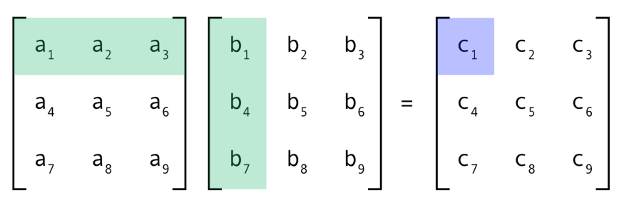
Figure 5.2: Matrix multiplication
we can use the %*% sign.
matrixA %*% matrixB## [,1] [,2] [,3]
## [1,] 84 90 96
## [2,] 201 216 231
## [3,] 318 342 366Finally, we can also test if something is a matrix by using the is.matrix() function. For example, if we do this with matrixA:
is.matrix(matrixA)## [1] TRUEthen we see that the result is TRUE again, which indicates that this is a matrix. There many more matrix operations, but we won’t go into that further because matrices will not be used very often in this book.
5.2.4 Data frame
We can also create data frames ourselves with the data.frame() function, but this is rarely done in practice. Generally, data frames are loaded by using, for example, SPSS or excel files. Later in the book, we will discuss data frames and loading data in greater detail. For the moment it’s useful to see a data frame once and know that we can create one similarly as we did with lists.
names <- c("Sarah", "Hugo", "James")
grades <- c(5, 8, 9)
pass <- c(FALSE, TRUE, TRUE)
example_dataframe <- data.frame(names, grades, pass)
example_dataframe
## names grades pass
## 1 Sarah 5 FALSE
## 2 Hugo 8 TRUE
## 3 James 9 TRUEIf we compare the output of this data frame to that of a list we see that with the list we only had one column of data and that they were separated with [[1]], [[2]], and so on. In contrast, a data frame can have multiple columns and rows of data. Again, we can also test if something is a data frame by using the is.data.frame() function.
is.data.frame(example_dataframe)## [1] TRUEAnd the output shows that this is indeed a data frame.